


Even for enthusiastic ML practitioners who are convinced that the more data the better, sometimes datasets are just too big for one-shot training. What is the best way to distill a large dataset into a smaller one, keeping relevant information for a specific ML task? We give an introduction to data selection methods and highlight situations where these methods enable ML models to learn better.
The set of techniques designed to select the most representative portion of a dataset for a specific task at a given size is called active sampling. It is meant for situations where pruning datasets is critical (see some examples in our previous post on random sampling). We’ll look closely at methods that select relevant samples, based on uncertainty, predictive loss, and gradients. After following this article, you will have:
- An intuition of how advanced active sampling techniques work, and
- A grasp of high-data/low-budget situations, where advanced data pruning is most beneficial.
Active Sampling: Keep the Most Relevant Samples
The idea behind active sampling is that an ML model doesn’t need to learn from all data, but only samples relevant for the task are truly necessary. For instance, noisy samples, with incorrect labels or that are simply uninformative, should be avoided. The same goes for outliers, which could add bias to the model, or redundant samples, for which few prototypes are enough.
Active sampling strategies have been introduced mainly for deep learning models and visual datasets, and are thus naturally designed to be part of the iterative training process of deep learning models. We can represent them as scoring functions (figure below) that assign a relevance score to every sample in the training set to finally select the most relevant batch to train on. As the model is updated at a new iteration, the scoring function is applied again to rank the full set and select a new batch.
Active sampling ranks dataset samples via relevance scores to select the most representative subset of data to train ML models.
If you are familiar with active learning (have a look at our previous post), this relevance score must ring a bell. Both active learning and sampling aim to select the most relevant samples for a predictive task, but the former ranks unlabeled samples, to select the best subset for annotation, while the latter ranks labeled samples to select the best subset for training. With labels, the active sampling scoring functions capture richer information about the sample relevance, such as the error, the loss, and its gradients, which could not be computed in active learning.
Active sampling methods identify the most representative subset of the training data, called the coreset, by guaranteeing that models that fit the coreset also provide a good fit for the original data. To obtain such coreset C* and its sample weights 𝛾, we need to solve an optimization problem, looking for the subset that best preserves the performance metric M, with respect to the same metric computed on the entire dataset D (up to a user-chosen tolerance ε).
Depending on the method, the metric can be a performance metric, such as the validation loss, or other proxy metrics, such as the average gradient of the validation set.
In practice, active sampling methods boil down to scoring functions assigning a relevance score to rank each sample. But how do we score samples by relevance? How do we find this coreset?
In active sampling, the relevance of a sample is encoded using various types of information:
- Geometry: A sample that is in a dense region and far away from other samples already selected is likely to be relevant.
- Uncertainty: A sample that the model is not confident to predict is probably a hard sample that is worth learning, while a sample the model can predict with very high confidence is probably redundant.
- Error (or loss): If a model can’t predict a sample correctly, it probably means that this is a hard sample that is worth learning or maybe a noisy sample to be discarded with a different technique.
- Gradient: The larger the gradients of the model loss with respect to its parameters, computed for a sample, the more this sample will impact the model, as the update directly depends on the gradients. Thus, we can assume that a sample that produces large gradients is relevant and worth learning.
All techniques except the geometry-based require an ML model to score samples. This is a sort of a paradox, as we don’t have an ML model to use to start with, on the contrary we are in the process of selecting the training set for our model-to-be. To solve this, researchers propose to train small proxy models on a small randomly selected pool of data (see figure below). This poses many difficult questions:
- How do you choose the proxy model?
- How large should the initial pool of data be?
- Can the proxy model (for selection) be different from the end predictive model?
Some active sampling techniques make use of initial proxy models to build relevance scoring functions.
We tried to answer those questions, playing with some of the latest coreset methods. Let’s zoom into some of them.
Uncertainty Margin:
The difference between the probability of the predicted class and the second-highest predicted probability is a measure of the model confidence. This difference is called margin, and its complement is a common metric for the uncertainty of the model regarding its prediction.

Rholoss (Reproducible Holdout loss) [1]:
The training loss for a specific sample measures how difficult it is for the model to predict it, but the training loss alone can be high for outliers also (i.e., noisy, ambiguous samples that should actually be discarded). In order to underrate them, the Reducible Holdout loss (or Rholoss) scoring function looks at the difference of two losses, the training loss and the irreducible holdout loss.
The former is the loss of a proxy model trained on a small portion of the training set, while the latter is the loss of an even simpler proxy model trained on a small holdout set (typically the validation set). All else being equal (with same training loss), the holdout loss is higher for noisy samples and outliers than for more relevant samples because these are less likely to be present in the holdout set used to train the holdout model.

GraNd (Gradient Normed) [2]:
This sampler requires differentiable models and it assigns a sample a relevance score based on the average of the gradient of the loss. It typically uses only the gradients of the parameters in the penultimate layer of the network (just before the linear layer, with softmax activation yielding the class probabilities).
The larger these gradients, the larger the update required on model parameters to learn a sample, meaning that this sample contains new and relevant information not yet taken into account. Improved versions average the individual scores obtained from an ensemble of models with different weight initializations (expectation over networks in the formula below). One interesting aspect of GraNd is that it can yield useful relevance scores even using the gradients of an untrained model.

In all these active samplers, we need one or two proxy ML models to produce the relevance score. We first choose an MLP for all of them, then study the impact of using different types of models.
The active sampling field is rich in other similar techniques. For a deep dive, have a look at [3].
All these active samplers have several limitations: First, they rely on time-consuming operations (training a proxy model on a small initial subset and inference on the whole, possibly very large, training set) that could sometimes make the data selection process very long. Secondly, relying on proxy models introduces many hyperparameters to tune, which largely affect the selection quality: model type and architecture, size of the initial training set and, for deep learning models, all the usual hyperparameters: the number of epochs, the learning rate, and so on.
In spite of these limitations, is active data selection better than simple and fast random sampling?
Comparing Active Samplers
The promise of active sampling is to break beyond the power scaling law typical of ML models learning curves under random sampling.
Theoretical results and experiments on simulated data in [4] highlight that advanced sampling techniques are only better than random sampling in a high-data/low-budget regime, which is when we have to sample a small coreset from a very large dataset (yellow 10% curve in the figure below).
In this regime (right side of the plot), the (black) learning curve, obtained by random sampling more training data, follows a power law (〜number_of_samples-1), while the (yellow) learning curve, obtained by active sampling the 10% of larger datasets, follows a steeper exponential law. The sampler used here is the EL2N, the precursor of GraNd, scoring the relevance of a sample by its error.
Learning curves can reach exponential scaling in high-data/low-budget scenarios. Power scaling with random sampling in black. Figure from [4].
The previous paper, like most of the literature in active sampling, is concerned with visual models. Thus, we tried out a few experiments to test active sampling techniques on tabular data, using six datasets that contain anywhere from 10,000 to 10 million samples (293/covertype, flight-delay-dataset, higgs, metropt_failures, tabular-playground-series-sep-2021, user_sparkify_event_data).
Depending on the dataset, we get some improvement in F1 metric when learning on the coreset instead of the random selection (for all the three active sampling methods), but this only happens in low-budget regimes. The larger the portion of the data we sample, the less important the gain over using simple random sampling is. You can see the results for four datasets below: The higher and steeper the learning curve, the better the selection method.
We observe two facts that are aligned with the picture above from [4]:
- For datasets with one million rows, if we select less than 10,000 samples (1% of the data), we get a benefit in using advanced samplers (moving from high-budget to low-budget);
- For smaller datasets, i.e., 500,000 rows (moving to low-data), random sampling is the best choice to select more than 500 samples (1‰ of the data).
F1-score learning curve of XGBoostingClassifier trained on four different datasets, where training subsets are selected via random sampling (black dotted line) or active sampling techniques (colored lines). Lines represent median value while the error band is the 90% confidence interval.
The GraNd and Rholoss active samplers successfully select data for training deep learning models for visual tasks. Here, with tabular data, we can see that simple uncertainty allows a more representative selection than random sampling and is more stable across datasets than Rholoss and GraNd. In addition, uncertainty is also faster than Rholoss and GraNd by one or two orders of magnitude (picture below), thus standing out as a selection method of choice for tabular data in high-data, low-budget regime.
In this experiment, all the hyperparameters of the active samplers have been optimized for an MLP proxy model, trained on an initial (randomly-sampled) training pool of 1,000 samples, on average. But the MLP is not really the most appropriate model when it comes to tabular data: Couldn’t we get better coresets using other types of models?
Average sampling time (s, log scale) of different samplers used to select portions up to 1% of the six datasets above.
The Importance of the Selection Model
We again compare the active sampling techniques above with random sampling, but this time using other types of proxy models, better designed for tabular data: an XGBoostingClassifier and a TabPFN [5].
For uncertainty and Rholoss samplers, we can compare the three types of proxy models (MLP, XGBoostingClassifier, and TabPFN), while for GraNd, which differentiable models, we can compare MLP and TabPFN. You can see from the results below, that actually the MLP is not such a bad choice, and that the gain with using XGBoostingClassifier or TabPFN is not that clear.
F1-score learning curve of XGBoostingClassifier trained on four different datasets, where training subsets are selected via random sampling (black dotted line) or an active sampling technique (uncertainty on the left and GraNd on the right). Colors show different selection models behind the active samplers.
Coresets in Hyperparameters Tuning
As hyperparameters tuning involves training hundreds or even thousands of models, speeding up individual training has an important benefit on the whole process. We saw in our previous post (experiment from [6]) that the relative performance of the HP configurations is roughly maintained, when the HP search is done training on small randomly sampled subsets of MNIST, instead of the full dataset. Do we observe this same behavior, when using actively sampled subsets, instead?
In the figure below, you can see the evaluation of an SVM model on a 10x10 lambda-gamma hyperparameters grid, realized using subsets of the MNIST dataset (1/128, 1/16, 1/4 and the entire dataset from left to right), where the subsets are sampled via GraNd. The blue region, which outlines the best configurations, is roughly maintained as we use less data, so that the result is very similar to what obtained via random sampling.
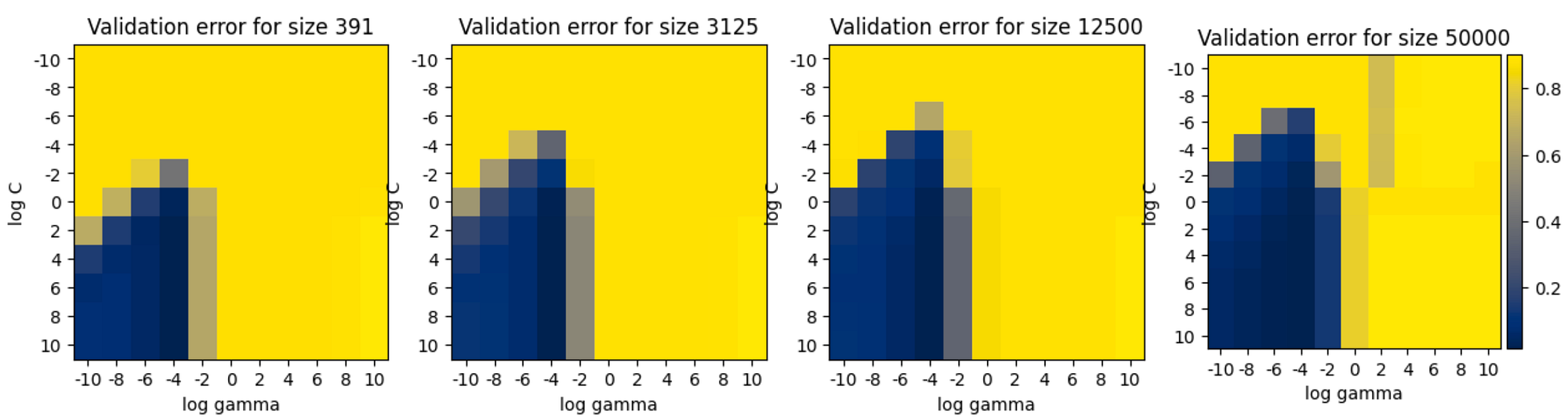
Validation error for 10x10 configurations of SVM hyperparameters gamma and lambda. The HP search is performed on subsets of MNIST dataset of size 1/128, 1/16, 1/4, and the entire dataset from left to right. The subsets are sampled via GraNd.
To have a quantitative estimation of the quality of the approximated HP search on subsets, we can look at the accuracy of the models when doing the grid search on the entire dataset (rightmost plot above) and the accuracy of the same HP configurations when doing the grid search on a subset (three leftmost plots above). For the approximated HP search to be of practical use, we need the correlation between these two sets of accuracies to be high.
You can see below the Kendall rank correlation coefficients between these accuracies (across fiveiterations), for randomly and GraNd-ly sampled subsets for 1/128, 1/16, 1/4 of the MNIST dataset. The Kendall correlation is chosen as we want the ranking between the accuracies to be roughly maintained, regardless of the accuracy values.
Although with the GraNd sampling we get more robust results for small subset sizes (reduced variance), in this simple experiment, correlations are very similar for the active and the random sampling. On the other hand, for more complex HP configurations, and especially when pruning from very large datasets, active sampling could improve the HP search on small subsets, identifying good configurations that are possibly missed when using random sampling.
Boxplots show the Kendall correlation (across five iterations) of the accuracy corresponding to HP configurations when using a subset (x-axis) with the final accuracy (training on the entire dataset).
Conclusion
With this article, you should have obtained an overview of advanced selection techniques in active sampling and how they can be extended to tabular data. As we have seen, active sampling has been designed to break beyond power law scaling of ML models’ performance with respect to the dataset size but, in practice, beating random sampling is hard.
While the dream of making models learn faster on less, but more relevant, data is very attractive, in our benchmark we observe that active sampling is mainly beneficial in situations where we need to select small batches from very large datasets.
References
[1] Prioritized Training on Points that are Learnable, Worth Learning, and Not Yet Learnt
[2] Deep Learning on a Data Diet: Finding Important Examples Early in Training
[3] DeepCore: A Comprehensive Library for Coreset Selection in Deep Learning
[4] Beyond neural scaling laws: beating power law scaling via data pruning
[5] TabPFN: a Transformer that solves small tabular classification problems in a second
[6] Fast Bayesian Optimization of Machine Learning Hyperparameters on Large Datasets