Clustering: How It Works (In Plain English!)

In the previous two posts in the How They Work (in Plain English!) series, we went through a high level overview of machine learning and took a deep dive into two key categories of supervised learning algorithms — linear and tree-based models. Today, we’ll explore the most popular unsupervised learning technique, clustering.

As a reminder, supervised learning refers to using a set of input variables to predict the value of a labeled output variable. Conversely, unsupervised learning refers to inferring underlying patterns from an unlabeled dataset without any reference to labeled outcomes or predictions.

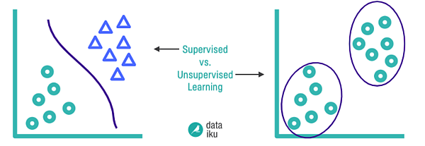
There are several methods of unsupervised learning, but clustering is far and away the most commonly used unsupervised learning technique, and will be the focus of this article. Clustering refers to the process of automatically grouping together data points with similar characteristics and assigning them to “clusters.”

Some use cases for clustering include:

• Recommender systems (grouping together users with similar viewing patterns on Netflix, in order to recommend similar content)
• Anomaly detection (fraud detection, detecting defective mechanical parts)
• Genetics (clustering DNA patterns to analyze evolutionary biology)
• Customer segmentation (understanding different customer segments to devise marketing strategies)

Clustering in Action: Practical Examples

If you missed the first post in this series, see here for some background on our use case. TL;DR let’s pretend we’re the owners of Willy Wonka’s Candy Store, and we want to perform customer segmentation. For each customer, we just have two data points: age and dollars spent at our store last week. Clustering will enable us to analyze the groups of consumers that purchase from our store, and then market more appropriately to each customer group.

If we had a very small dataset, we could do this manually by finding customers with similar features. For example, we may notice that there are three general groups of consumers:

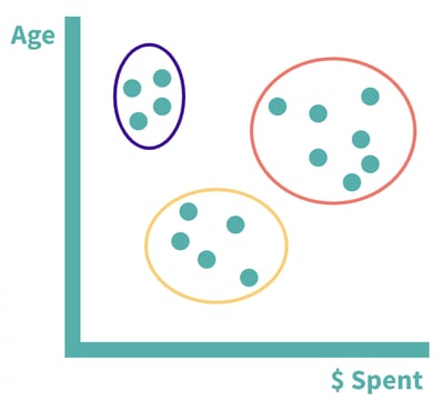
Similar data points occupy close spatial positioning. Group one is in purple, group two is in orange, and group three is in yellow.

This is of course a major over-simplification, and Willy Wonka Candy Store is much too popular of a store for such a simple consumer segmentation. This is where unsupervised learning comes in — we can let the algorithm find these groups for us automatically. Today, we’ll explore two of the most popular clustering algorithms, K-means and hierarchical clustering.

K-Means Clustering

K-means clustering is a method of separating data points into several similar groups, or “clusters,” characterized by their midpoints, which we call centroids.

Here’s how it works:

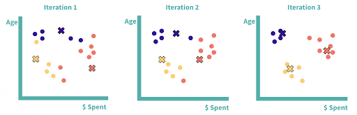
Three iterations of K-means clustering. After the third iteration, we have our final clusters — the centroids have stabilized, and the data points will no longer be reassigned.

Note that if we had more than two features in our model, this would become hard or impossible to visualize, but the concept remains the same — plot the data points in an N-dimensional space and measure the distance between them.

How do I select the number of clusters (K)?

Good question. The most common way to do this is by using what’s referred to as an elbow plot. You can build an elbow plot by iteratively running the K-means algorithm, first with K=1, then K=2, and so on, and computing the total variation within clusters at each value of K.

A common way of computing variation is by looking at the sum of squared distances from each point to its cluster center. If we ran K-means with only one cluster, we would have one huge cluster, so the within-cluster variance would be very high, and alternatively, if each cluster consisted of only one point, the total variation would be zero. As we increase the value of K and the number of clusters goes up, the total variation within clusters will necessarily decrease.

The goal of the elbow method is to find the inflection point on the curve, or the “elbow.” After this point, additional clusters do not minimize the within cluster variance significantly enough to justify additional groupings in the dataset. There is no hard and fast rule here, as it’s often up to the discretion of the data scientist, but looking at an elbow plot tends to be a good place to start.

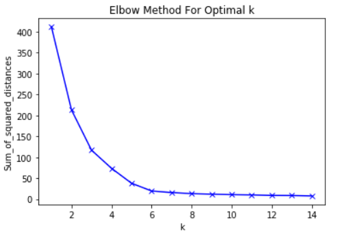
Elbow plot for sample data. Here, the elbow is at around five, so we may want to opt for five clusters.

Hierarchical Clustering

Hierarchical clustering is another method of clustering. Here, clusters are assigned based on hierarchical relationships between data points. There are two key types of hierarchical clustering: agglomerative (bottom-up) and divisive (top-down). Agglomerative is more commonly used as it is mathematically easier to compute, and is the method used by python’s scikit-learn library, so this is the method we’ll explore in detail.

Here’s how it works:

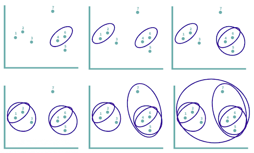
In this example, we’d start with seven clusters, and iteratively group data points together based on distance until all data points are finally merged into one large cluster.

With divisive hierarchical clustering, we’d start with all data points in one cluster and split until we ended up with each datapoint as its own cluster, but the general concept remains similar.

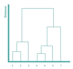
To visualize and better understand the agglomeration process, we can use dendrogram, which shows the hierarchical relationships between clusters. The taller the line, the greater the distance between two points. Because four and six were the closest and were merged first, those two are connected by the shortest lines. We can visualize the entire process laid out above in this dendrogram.

How do we measure the similarity between clusters?

There are a few different ways of measuring distance between two clusters. These methods are referred to as linkage methods and will impact the results of the hierarchical clustering algorithm. Some of the most popular linkage methods include:

1. Complete linkage, which uses the maximum distance between any two points in each cluster.
2. Single linkage, which uses the minimum distance between any two points in each cluster.
3. Average linkage, which uses the average of the distance between each point in each cluster.

Euclidean distance is almost always the metric used to measure distance in clustering applications, as it represents distance in the physical world and is straightforward to understand, given that it comes from the Pythagorean theorem.

How do we decide the number of clusters?

You can again use an elbow plot to compare the within-cluster variation at each number of clusters, from 1 to N, or you can alternatively use the dendrogram for a more visual approach. You can do so by considering each vertical line in the dendrogram and finding the longest line that is not bisected by a horizontal line. Once you find this line, you can draw a dotted line across, and the number of vertical lines crossed represents the number of clusters generated.

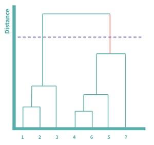
The longest line not bisected by a horizontal line has been colored orange. In this example, we’d have two clusters, one with 1, 2, and 3, and another with 4, 5, 6 and 7.

Recap

K-means and hierarchical clustering are both very popular algorithms, but have different use cases. K-means tends to work much better with larger datasets, as it’s relatively computationally efficient. Hierarchical clustering, on the other hand, does not work well with large datasets due to the number of computations necessary at each step, but tends to generate better results for smaller datasets, and allows interpretation of hierarchy, which is useful if your dataset is hierarchical in nature.

As with almost any machine learning problem, there’s no one-size-fits all solution, but these two algorithms each have different use cases, and it’s important to consider the nature of your dataset when deciding which algorithm to use.