


Previously, we investigated the differences between versions of the gradient boosting algorithm regarding tree-building strategies. We’ll now have a closer look at the way categorical variables are handled by LightGBM [2] and CatBoost [3].
We first explain CatBoost’s approach for tackling the prediction shift that results from mean target encoding. We demonstrate that LightGBM’s native categorical feature handling makes training much faster, resulting in a 4 fold speedup in our experiments. For the XGBoost [1] adepts, we show how to leverage its sparsity-aware feature to deal with categorical features.


The Limitations of One-Hot Encoding
When implementations do not support categorical variables natively, as is the case for XGBoost and HistGradientBoosting, one-hot encoding is commonly used as a standard preprocessing technique. For a given variable, the method creates a new column for each of the categories it contains. This has the effect of multiplying the number of features that are scanned by the algorithm at each split, and that is why libraries such as CatBoost and LightGBM implement more scalable methods.
Processing of Categorical Variables in CatBoost
Ordered Target Statistics Explained
CatBoost proposes an inventive method for processing categorical features, based on a well-known preprocessing strategy called target encoding. In general, the encoded quantity is an estimation of the expected target value in each category of the feature.
More formally, let’s consider the category i of the k-th training example. We want to substitute it with an estimate of

A commonly used estimator would be
which is simply the average target value for samples of the same category as xⁱ of sample k, smoothed by some prior p, with weight a > 0. The value p is commonly set to the mean of the target value over the sample.
The CatBoost [3] method, named Ordered Target Statistics (TS), tries to solve a common issue that arises when using such a target encoding, which is target leakage. In the original paper, the authors provide a simple yet effective example of how a naive target encoding can lead to significant errors in the predictions on the test set.
Ordered TS addresses this issue while maintaining an effective usage of all the training data available. Inspired by online algorithms, it arranges training samples according to an artificial timeline defined by a permutation of the training set. For each sample k from the training set, it computes its TS using its own “history” only; that is, the samples that appear before it in the timeline (see example below). In particular, the target value of an instance is never used to compute its own TS.
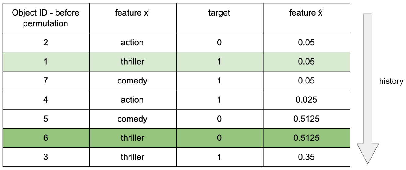
Values of x̂ⁱ are computed respecting the history and according to the previous formula (with p = 0.05). In the example of Table 3, x̂ⁱ of instance 6 is computed using samples from its newly assigned history, with x̂ⁱ = thriller. Thus, instance 1 is used, but instance 3 is not.
In the CatBoost algorithm, Ordered TS is integrated into Ordered Boosting. In practice, several permutations of the training set are defined, and one of them is chosen randomly at each step of gradient boosting in order to compute the Ordered TS. In this way, it compensates for the fact that some samples TS might have a higher variance due to a shorter history.
A Few Words on Feature combinations
In addition to Ordered TS, CatBoost implements another preprocessing method that builds additional features by combining existing categorical features together. However, processing all possible combinations is not a feasible option as the total grows exponentially with the number of features. At each new split, the method only combines features that are used by previous splits, with all the other features in the dataset. The algorithm also defines a maximum number of features that can be combined at once, which by default is set to 4.
Native Support of Categories in LightGBM
LightGBM provides direct support of categories as long as they are integer encoded prior to the training. When searching for the optimal split on a particular feature, it will look for the best way of partitioning the possible categories into two subsets. For instance, in the case of a feature with k categories, the resulting search space for the algorithm would be of size 2ᵏ⁻¹–1.
In practice, the algorithm does not go through all possible partitions and implements a method derived from an article from Fisher [4] (On Grouping for Maximum Homogeneity — 1958) to find the optimal split. In short, it exploits the fact that if the categories are sorted according to the training objective, then we can reduce the search space to contiguous partitions. This significantly reduces the complexity of the task.
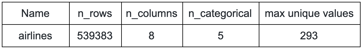
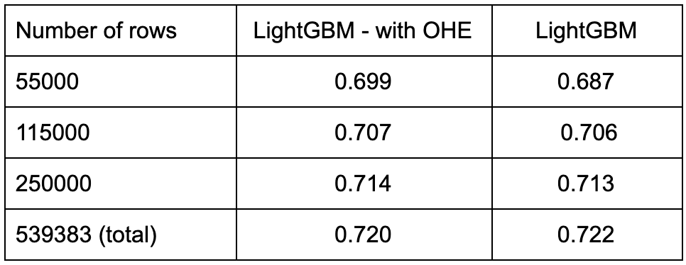
In the experiment below, we investigate the benefits of using categorical feature handling instead of one-hot encoding. We measure the mean fit time and best test scores obtained with a randomized search on subsets of different size of the airlines dataset. This dataset, whose statistics are summarized in Table 2, contains high cardinality variables which make it suitable for such a study.
The results show that both settings achieve equivalent performance scores, but enabling the built-in categories handler makes the LightGBM faster to train. More precisely, we achieved a 4 fold speedup on the full dataset.
Dealing with Exclusive Features
Another innovation of LightGBM is Exclusive Feature Bundling (EFB). This new method aims at reducing the number of features by bundling them together. The bundling is done by regrouping features that are mutually exclusive; that is, they never (or rarely) take non-zero values simultaneously. In practice, this method is very effective when the feature space is sparse, which, for instance, is the case with one-hot encoded features.
In the algorithm, the optimal bundling problem is translated into a graph coloring problem where the nodes are features and edges exist between two nodes when the features are not exclusive. The problem is solved with a greedy algorithm that allows a rate of conflicts 𝛾 in each bundle. With an appropriate value for 𝛾, the number of features (and thus the training time) are significantly reduced while the accuracy remains unchanged.
How does EFB Affect Scalability?
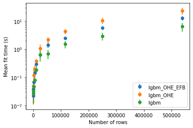
We investigated the importance of EFB on the airlines task. In practice, we did not notice any effect of EFB on fit time when using the categorical feature handler of LightGBM. However, EFB did improve the training time by leveraging the sparsity introduced by OHE as shown in Figure 2. The results with categorical feature handling enabled (lgbm) are shown as a reference point.
Tweaking XGBoost’s missing value handler
XGBoost does not support categorical variables natively, so it is necessary to encode them prior to training. However, there exists a way of tweaking the algorithm settings that can significantly reduce the training time, by leveraging the joint use of one-hot encoding and the missing value handler !
XGBoost: A Sparsity-Aware Algorithm
In order to deal with sparsity induced for instance by missing values, the XGBoost split-finding algorithm learns from the data at each split a default direction for these values. In practice, the algorithm tests two possible grouping for the instances with missing values (left and right), but these points are not visited one by one like the others. This saves a lot of computations when the data is very sparse.
What is interesting is that this particular feature is not limited to missing values as we usually understand them. In fact, you can choose any constant value you want to play the role of missing value, when your data does not contain any. This becomes very handy when working with datasets for which one-hot encoding introduces many zeros entries.
Leveraging the sparsity introduced by one-hot encoding
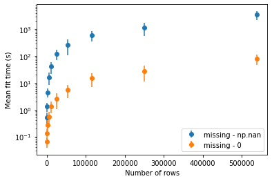
We investigated the importance of setting the missing parameter of the split-finding algorithm to 0 (instead of numpy.nan, the default value in the Python implementation), on the training of the airlines dataset. The results reported in the figure below are for the approx tree-building method, but the same observations were made for exact and hist.
Changing the missing parameter to 0 results in a significant reduction of training time. More precisely, we observed a 40× speedup for exact and approx on the full dataset, and a 10× speedup for hist.
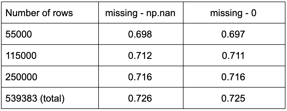
As shown in Table 4, this small change does not seem to affect the performance scores in any significant way, making it a practical tip for when working with datasets with no actual missing data.
Takeaways
Because of the way Gradient Boosting algorithms operate, optimizing the way categorical features are handled has a real positive impact on training time. Indeed, LightGBM’s native handler offered a 4 fold speedup over one-hot encoding in our tests, and EFB is a promising approach to leverage sparsity for additional time savings.
Catboost’s categorical handling is so integral to the speed of the algorithm that the authors advise against using one-hot encoding at all(!). It is also the only gradient boosting implementation to tackle the problem of prediction shift.
Finally, we demonstrated that in the absence of true missing data, it is possible to leverage XGBoost’s sparsity aware capabilities to gain significant speedups on sparse one hot encoded datasets, achieving up to a 40× speedup on the airlines dataset.
References
[1] Chen, T. & Guestrin, C. XGBoost: A scalable tree boosting system. Proc. ACM SIGKDD Int. Conf. Knowl. Discov. Data Min. 13–17-Augu, 785–794 (2016).
[2] Ke, G. et al. LightGBM: A highly efficient gradient boosting decision tree. Adv. Neural Inf. Process. Syst. 2017-Decem, 3147–3155 (2017).
[3] Prokhorenkova, L., Gusev, G., Vorobev, A., Dorogush, A. V. & Gulin, A. Catboost: Unbiased boosting with categorical features. Adv. Neural Inf. Process. Syst. 2018-Decem, 6638–6648 (2018).
[4] Walter D. Fisher (1958) On Grouping for Maximum Homogeneity, Journal of the American Statistical Association, 53:284, 789–798, DOI: 10.1080/01621459.1958.10501479