How to Measure Dataset Similarity: Understanding the Impact of Drift on ML Models

Measuring similarity between two datasets is critical in many ML fields, such as detecting dataset shift and evaluating its impact on a model’s performance. This article describes various datasets’ similarity measures and how they can be leveraged for distribution shift detection and model performance drop.

Similarity measures are used in a wide range of applications such as meta-learning (where we need to select diverse datasets to train models to generalize to new datasets), domain adaptation (where we are interested in finding a subset of training data more similar to a new dataset), or transfer learning, where we want to select the closest pre-training data and augmentations to a new dataset.

TL;DR: Some similarity measures such as the proxy-A-distance (PAD) are suitable to detect shifts due to corrupted data. However, they do not stand out when predicting the model’s performance drop where the Maximum Mean Discrepancy (MMD) applied on embeddings and the Wasserstein distance on images are much more efficient. When the purpose is to compare datasets from a classification perspective, optimal transport that takes into account labels reliably expresses the resemblance of the predictive tasks that datasets represent.

ImageNet-C: A Corrupted Visual Dataset for a Robustness Benchmark

ImageNet-C is a visual dataset built upon the infamous ImageNet dataset to test neural networks’ robustness to corruptions and perturbations. We will use it to simulate dataset shift or drift, a thorn in the side of ML in production, which is a change of distribution in new data that can possibly lead to a drop in performance of deployed ML models (more on drift).

This dataset consists of 18 different corruptions: different noises, blur effects, weather effects (fog, snow, frost), etc. Each corruption is parametrized by five levels of severity.

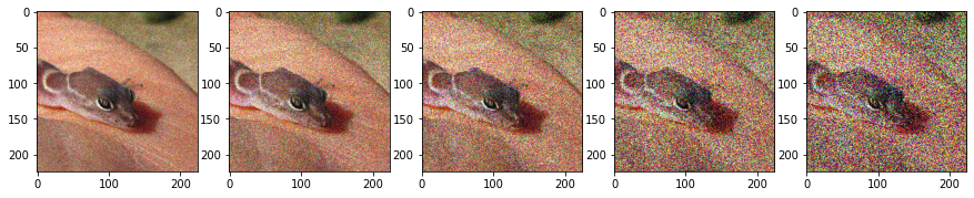
Five levels of severity of shot noise on one image

This article focuses on noise corruptions that simulate data shifts that occur during three different stages of a visual task pipeline: Gaussian noise that appears in low lighting conditions; shot noise, an electronic noise due to the discrete nature of the electric charge; and speckle noise, a numeric noise occurring with byte-encoding errors.

In our MLOps scenario, the clean ImageNet is the source dataset used to train ML models, while the various corruptions represent target datasets under shift.

We use a ResNet-50 pretrained on ImageNet as the model deployed in production and compute its actual performance drop on various corruptions and with different levels of severity (0 meaning no corruption).

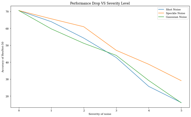
Performance drop due to different noises on a ResNet-50

As we can see above, there is a clear drop in a model’s performance, especially at high severity. The baseline performance of the ResNet-50 is 70% on the test set. It then quickly decreases below 20% for severity five.

True performance drop is unknown in real life as we have no labels for the incoming target data. In order to detect potential shifts and then estimate their impact on the performance of our model, we need metrics that indicate how far the incoming data is from the original data. Let us explore some of them.

Measuring Similarity Between Datasets' Features

We start by considering measures of similarity between datasets without considering their labels. As the incoming data is not labeled, shift can only be detected in an unsupervised fashion.

We present three metrics: the PAD, the MMD, and the Wasserstein distance.

The PAD: The PAD is defined following a simple and intuitive methodology. First, mix source and target datasets and label them according to the origin of each sample (0 for the first dataset, 1 for the second). Then, train a domain classifier on merged data, test it on the held-out test set, and note 𝜖 its error. Finally, we can define the PAD as:

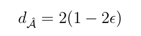
If the two datasets’ distributions are similar, the domain classifier will not be able to discriminate between them; its accuracy will be around 50%, and its PAD will be zero. If the classifier has high accuracy, it can easily recognize the target dataset. Hence, source and target datasets may not follow the same distribution, revealing a dataset shift.

Even if PAD is the theoretical definition of this metric, we use only the accuracy of the domain classifier in practice.

Here is a simple implementation of this metric:

If the domain classifier needs to be retrained for every new batch of data, it can indicate the most anomalous samples by their predicted probability of belonging to the original dataset.

MMD: The underlying idea behind MMD is to represent the distance between distributions as the distance between mean embeddings of their features.

With P, Q distributions, X, Y realizations, and 𝜙 a feature map, it is defined as:

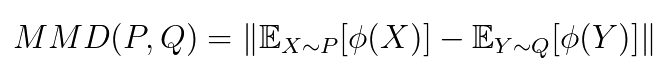
The underlying idea is to map the distribution to more expressive embeddings. For example, 𝜙(x) = (x, x2) will distinguish distributions with different variances and not only different means. In practice, we can generalize this idea with a more complex feature map that embeds our data in a high — potentially infinite — dimensional space.

Wasserstein Distance: The Wasserstein distance is based on the optimal transport problem [7]. With P and Q two distributions on 𝒳, c(.,.) a cost function and 𝛱(P, Q) the set of couplings between the distributions, we can define the optimal transport problem as:

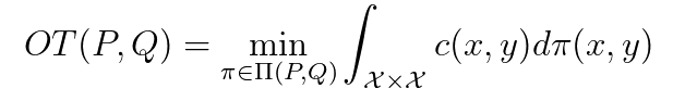
Intuitively, the cost function is the cost of transporting a unit of mass of x to y and 𝛱 the possible transport plans. If the cost function is the Euclidean distance, the optimal transport is called the Wasserstein distance. The Wasserstein distance has the advantage of leveraging the natural geometric properties of the space but is computationally expensive.

For MMD and Wasserstein distance, we used the package geomloss, which provides efficient GPU implementation of these metrics. Note: These similarity measures are sometimes referred to as distances. However, they are not all regular statistical distances and do not satisfy all the inherent properties (see Wikipedia).

Estimating Performance Drop and Shift Severity

We now see how well the above similarity measures can estimate performance drop under shift on ImageNet-C.

We trained a ResNet-50 on the clean and corrupted images as a domain classifier to estimate the PAD and achieved excellent discrimination (see below).

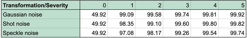
Accuracy of the domain classifier on corrupted data (The values of accuracy and all other metrics are averaged across multiple bootstrapped datasets)

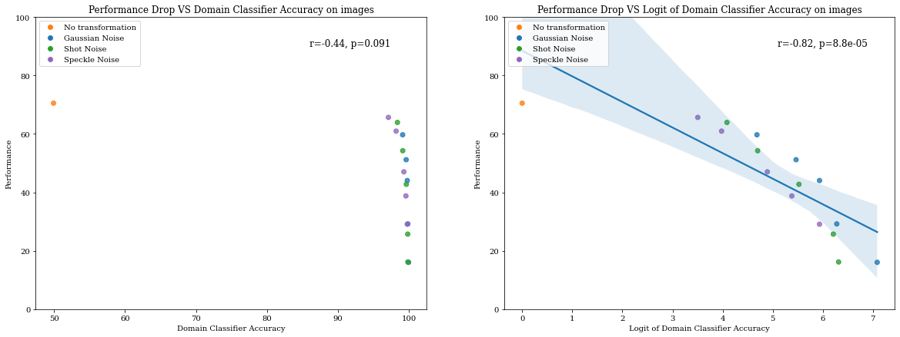
The correlation between the performance drop of the model and the accuracy of the domain classifier is medium (r=-0.44) because there is a considerable gap in domain classifier accuracy between the clean and corrupted datasets even at low severity, which is not apparent in model performance. However, by applying a logit transformation to the accuracy of the domain classifier, we can define another metric that correlates better with performance drop (r=-0.82).

We now test the MMD and the Wasserstein distances on the same task. We can compute those similarity measures both on the input space, the images (using pixels as features), or on the latent feature space, the embeddings extracted from a neural net (in our case, a ResNet-50 2048-dimensional embedding). We tried both approaches to highlight how sensitive MMD and Wasserstein distances are to the choice of the representation.

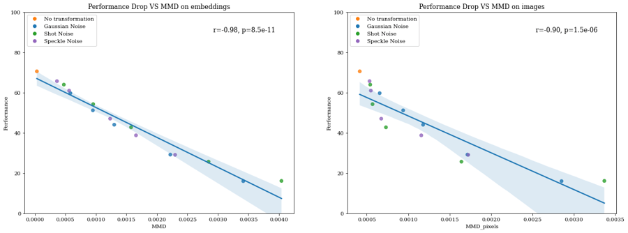
We observe above that MMD correlates better with performance drop using embeddings (r=-0.98) than pixels (r=-0.90).

However, the Wasserstein distance correlates better with raw images (r=-0.98) than with extracted embeddings (r=-0.5). As for the domain classifier, the Wasserstein distance on embeddings distinguishes easily between clean and corrupted datasets but is a bad proxy for performance drop.

In conclusion, we observe that:

• Domain classifier and Wasserstein distance on embeddings help detect dataset shifts but struggle to predict their severity and the following performance drop.
• MMD on embeddings and Wasserstein distance on images correlate well with the performance drop over various corruptions.

It suggests that we could directly employ similarity metrics from multiple synthetically generated corruptions to predict the performance drop in real shift scenarios reliably.

If target labels are often unavailable for instance in shift detection tasks, we have access to labeled samples in other tasks such as transfer learning. Ignoring the labels might lead us to believe that datasets are similar when they’re pretty different from a task perspective. It is then natural to rely on similarities between both features and label distributions.

Measuring Distances Between Tasks

Recent work considers the labels when measuring the dis(similarity) between two datasets and is an extension of the above optimal transport distance: The Optimal Transport Dataset Distance (OTDD).

The Optimal Transport Dataset Distance:

In addition to the metric on the features, it defines a label-to-label distance. To put it shortly, it fits a Gaussian distribution on the feature space (input or latent) for each label. Then, it computes once again a Wasserstein distance between two distributions associated with each pair of labels. The ground cost function combines the Euclidean distance on the features and the Wasserstein distance on the label distributions.

For a deeper dive into this approach, check the excellent blog post from Microsoft on the topic.

Why use distances on both features and labels?

We show an example where OTDD captures differences missed by regular optimal transport distances. We create three datasets from ImageNet, keeping only a subset of ten classes:

• A clean dataset without transformation
• A rotated dataset where we apply a rotation of 5° to all images
• A mixed-up dataset where half of the labels are set randomly among the ten classes

Intuitively, the clean and the rotated dataset distributions must be very similar as the images are only rotated by a slight angle. In terms of classification, their tasks are also very similar. On the other hand, the mixed-up dataset has little to do with the clean dataset in terms of classification, as the tasks are quite different.

We compute the Wasserstein and OTDD distances between the two perturbed datasets and the clean reference.

Distance between clean and rotated/mixed-up datasets (scaled to the distance between the clean dataset and itself)

As expected, the distance between the Wasserstein distance is more significant with the rotated dataset than with the mixed-up dataset. Indeed the distance between the features increases when rotating the dataset as mixing the labels does not change anything on the feature’s distance. However, swapping the labels increases the label-to-label distance on the OTDD by modifying their associated distributions.

This type of distance is helpful in a transfer learning setting. Imagine you have a classification dataset with few labeled samples. You would prefer transfer learning instead of training a model from scratch. However, rather than randomly choosing the dataset on which the model has been pretrained, one can determine the most similar one and use a model pretrained on it as a backbone. In addition, with these distances, you can choose the data augmentations that will make your source dataset the closest possible to your target dataset.

Key Takeaways