


This is the story of a research project that didn’t quite make it. As every research project, it started with what seemed like a good and natural idea. As with most research projects, it didn’t end up as groundbreaking work.
It wasn’t a catastrophic failure either. We believe that our method improves upon existing works, but too marginally to comply with the expectations of the research community. However, we believe there is value in sharing this universal journey of a research project!
Inspired by the original NeurIPS workshop
At the Dataiku AI Lab, we are interested in developing pragmatic research that can benefit all ML practitioners in their journey with data. This journey often starts with data that needs labeling and, as such, a first question naturally arises:
How can you most efficiently label data?
One way to tackle this very broad question is within the active learning framework, which has been of prime interest to our team lately.
The starting point. In 2019, Amazon proposed a query sampling strategy that combines both uncertainty estimation and diversity using a weighted K-Means algorithm called WKMeans. As French practitioners, we tend to think that the best dishes are cooked in old pots and were very seduced by this method capable of achieving state-of-the-art performance using the tried-and-tested K-Means. We even proposed a reproduction of their paper results in a previous blog post.
All Samples Are Not Made Equal
In our paper studying the properties of query sampling strategies published at ICDMW last year, WKMeans clearly leads the way in terms of performance. In order to explain why, we first need to explain the concept of sample (un)certainty.
In active learning, the value of a sample is equal to its capacity to change the prediction of other samples (like test samples) toward the right label. We expect this capacity to be correlated to the capacity of the sample to change its own prediction. Therefore, one of the first query strategies consists of selecting the samples with the lowest maximum predicted probability among classes as they have more room for growth.
Mathematically, we can formulate the potential gain of a sample at iteration i as the difference between its current predicted probability using classifier h, and its ideal predicted probability that we would only reach after an infinite amount of iterations:

If a sample already has a high predicted probability, there is no improvement to expect: those are easy-to-classify samples as illustrated here. The bad performance of purely exploratory sampling strategies, such as K-Means, can be explained by their focus on easy samples.
On the other side of the spectrum, there is a category of samples usually disregarded in active learning: the hard-to-classify samples for which the maximum probability is very low (say because it is a dog that looks like a muffin). The bad performance of entropy sampling on the CIFAR100 dataset for instance can be explained by its selection of mostly hard-to-classify samples. In our study, we observe that WKMeans selects samples in a sweet spot that are not too easy nor too hard to classify.
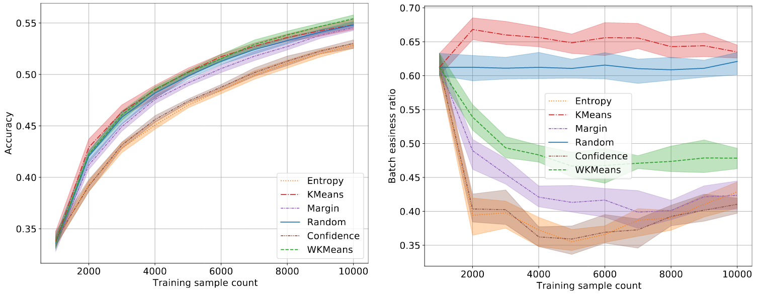
Accuracy and easiness to classify measured on CIFAR100. Confidence-based sampling selects hard samples while K-Means selects easier ones.
In fact, WKMeans performs a preselection of β * k samples with highest uncertainty to get rid of the easy-to-classify samples. Note that the selection process for this β parameter is not an easy task and has dramatic consequences: a value of β being too high can introduce easy-to-classify samples in the preselection. If this happens, the subsequent K-Means plays against us: instead of promoting diversity it will almost surely select some samples in the easy-to-classify region.
The Hard-to-Classify Honey Pot
In each task, some samples may be wrongly classified or so hard to classify that deriving a general rule for them is complex. Instead of bringing information, these samples can blur the boundary between two classes. Query sampling methods focusing on uncertainty estimation are very prone to select those samples because they may show high uncertainty even if similar samples are selected and labeled. Amazon’s proposed method is not immune to this problem since nothing prevents one sample from being selected next to an already labeled (and potential hard-to-classify) one.
Experiment. This problem is easy to spot using a synthetic dataset. For this purpose, we make use of the excellent make_blobs method from scikit-learn. We use it to generate blobs of data belonging to different classes, but we also generate noisy blobs where points are randomly attributed to two different classes, making them impossible to classify. In this setting, we expect uncertainty-based methods to fail by focusing on the noisy blobs. The method that we will introduce, IWKMeans, seems to be less affected by those blobs.
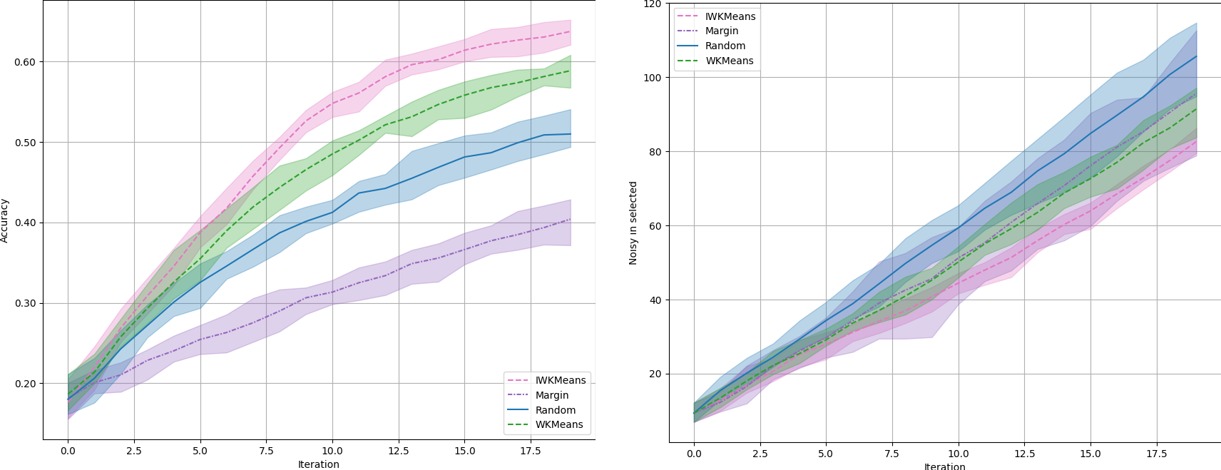
Accuracy on a synthetic dataset with 2 features, 10 classes, and 10,000 samples, of which 50% are noisy.
Killing 2 Birds With 1 Stone: Incremental WKMeans
How can we prevent our query sampling strategy from selecting samples that are too easy or too hard to classify? The first idea we got was simply to prevent the selection of samples nearby already selected ones, similarly to what Du did by maximizing the distance between the already selected samples and the ones in the batch. Let us detail how to implement this in WKMeans.
At a high level, the goal of batch active strategies is to select a batch of samples 𝔹 where uncertainty is high, but that is also representative of the unlabeled data 𝔹 ∼ 𝕌 and diverse. For a given notion of similarity “sim” between sets of samples, this leads to the following objective:

In Amazon’s method, the similarity measure is defined as follows:
 A natural proxy for this maximization is given by the K-Means objective. The above objective does not take into account the already labeled data and can lead to suboptimal batches lying in regions with a high-density of labeled samples. A natural refinement is to additionally impose that the selected batch differs from already labeled data 𝕃, i.e. to minimize the similarity sim(𝔹, 𝕃):

Within Amazon’s settings, this can be achieved by simply modifying the similarity in the objective to:
 Consequently, we propose to modify the K-Means procedure by adding fixed clusters corresponding to previously labeled samples in its objective. However, we do not select samples in these clusters: they act as repulsive points and prevent the procedure from selecting samples nearby already selected ones. We refer to this approach as Incremental WKMeans. Our implementation is available here.
Note that the use of this method is not limited to active learning. We use the incremental K-Means over iterations, but it could be used sequentially in order to build a hierarchical K-Means algorithm that allows us to control the number of clusters at each level.
In the synthetic problem presented above, we see that IWKMeans clearly dominates the other methods. It is also the one that selects the least noisy samples. Let us now see if this behavior is well transposed in real life datasets.
The Complicated Path to Real-Life Improvements
If the results on our synthetic dataset seem idyllic, they suffer from dire limitations. First, 50% of noisy data is a lot of noise and, in contexts with less noise, IWKMeans performs as good as WKMeans. We have also chosen to take two features and, again, the advantage of IWKMeans becomes less important with more dimensions, as shown below with 40 features.
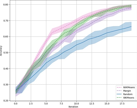
Let us now apply it on real-life data! On our reference tabular dataset, LDPA, IWKMeans brings a marginal improvement compared to WKMeans. Unfortunately, IWKMeans is equivalent to WKMeans in the rest of our suite of tasks (see CIFAR10 results on the right).
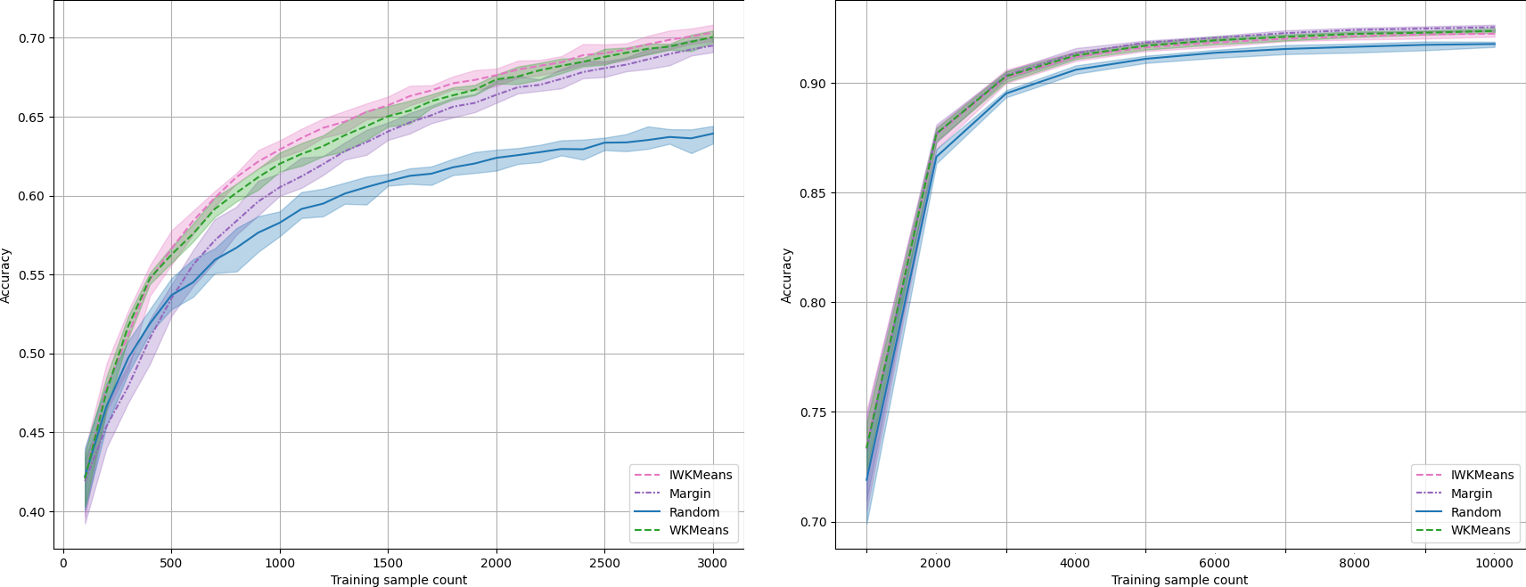
Accuracy on LDPA (left) and on CIFAR10 (right).
Robustness to β parameter. We observed some positive signals: the procedure seems to be more robust to the β parameter as originally hoped. This is due to the fact that when easy-to-classify samples are preselected, IWKMeans manages to discard them. On LDPA, we observe that IWKMeans with β at 10 and 80 perform the same, while WKMeans suffers from a degradation of performances (see figure below). Unfortunately, this effect does not generalize to CIFAR.
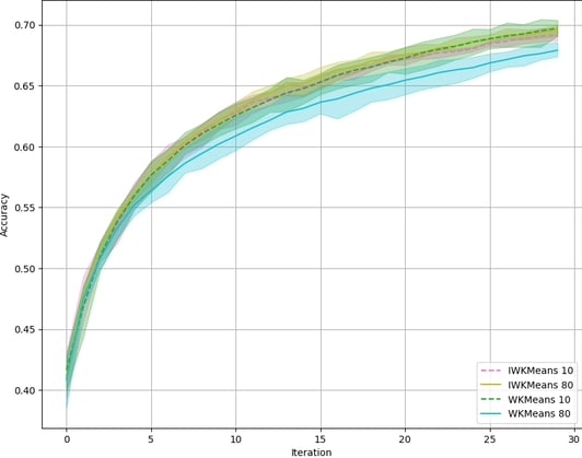
Accuracy for WKMeans and IWKMeans with β=10 and β=80 on LDPA.
Is IWKMeans converging properly? One could ask if the fixed cluster centers could prevent IWKMeans from converging. In particular, it is easy to conceptualize in 2D that some fixed clusters could prevent a moving cluster to reach its best position, as presented in the figure below. We checked and stated that if this can happen in 2D, it is not the case in higher dimensions. K-Means++ initialization also prevents it from happening. We have even tried not to fix the clusters but to reposition them on the fixed position from time to time, and it does not change the performance. See this example for more details.
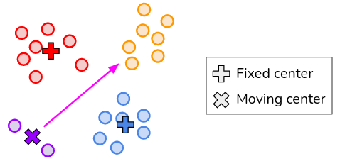
The moving purple center cannot reach its optimal position in the orange cluster because of the fixed red and blue centers.
Is IWKMeans preventing the selection of interesting points? IWKMeans prevents the selection around already labeled samples, whether they are too hard or too easy to classify. This approach is questionable with regards to the active learning intuition that is to explore the classifier’s decision boundary. Following this, we may want to prevent exploration nearby well-classified samples, but keep exploring the neighborhood of samples that are not well classified. For this purpose, we have created a variant of IWKMeans where we consider repulsive points the only labeled samples that are correctly classified by the model... The results are indistinguishable from the original version.
Conclusion
In the end, the cold hard truth is the IWKMeans performs very similarly to WKMeans.
Despite some promising signals in a restricted number of cases, IWKMeans needs more adjustments to be proven useful. In particular, we have observed that some of our intuitions about this algorithm hold well in low-dimension and simple classification use cases, but become less clear on complex and real-life use cases. In CIFAR 10, for example, blacklisting already labeled samples when exploring the airplanes versus cats boundary brings value, but doing it for dogs versus cats leads to suboptimal results. This is why margin sampling, which deeply explores the latter, manages to beat IWKMeans. In a further version of our algorithm, we want to explore the confusion matrix to have a behavior adapted to each problem. This may require going a bit further away from the original Amazon approach.