In our previous article, we gave an in-depth review on how to explain biases in data. The next step in our fairness journey is to dig into how to detect biased machine learning models.
 If only measuring fairness was that easy
However, before detecting (un)fairness in machine learning, we first need to be able to define it. But fairness is an equivocal notion — it can be expressed in various ways to reflect the specific circumstances of the use case or the ethical perspectives of the stakeholders. Consequently, there can’t be a consensus in research about what fairness in machine learning actually is.
In this article, we will explain the main fairness definitions used in research and highlight their practical limitations. We will also underscore the fact that those definitions are mutually exclusive and that, consequently, there is no “one-size-fits-all” fairness definition to use.
Notations
To simplify the exposition, we will consider a single protected attribute in a binary classification setting. This can be generalized to multiple protected attributes and all types of machine learning tasks.
Throughout the article, we will consider the identification of promising candidates for a job, using the following notations:
- 𝑋 ∈ Rᵈ: the features of each candidate (level of education, high school, previous work, total experience, and so on)
- 𝐴 ∈ {0; 1}: a binary indicator of the sensitive attribute
- 𝐶 = 𝑐(𝑋, 𝐴) ∈ {0; 1}: the classifier output (0 for rejected, 1 for accepted)
- 𝑌 ∈ {0; 1}: the target variable. Here, it is whether the candidate should be selected or not.
- We denote by 𝐷, the distribution from which (𝑋, 𝐴, 𝑌) is sampled.
- We will also note 𝑃₀(𝑐) = 𝑃(𝑐|𝑎 = 0)
The Many Definitions of Fairness
Unawareness
It defines fairness as the absence of the protected attribute in the model features.
Mathematically, the unawareness definition can be written as follows:

Because of this simplicity, and because implementing it only needs to remove the protected attribute from the data, it is an easy-to-use definition.
Limitations. Unawareness has many flaws in practice, which make it a poor fairness definition overall. It is far too weak to prevent bias. As explained in our previous article, removing the protected attribute doesn’t guarantee that all the information concerning this attribute is removed from the data. Moreover, unaware correction methods can even be less performant when it comes to fairness improvement than aware methods.
Demographic Parity
It stipulates that the predictions’ distribution should be identical across subpopulations.
Mathematically speaking, demographic parity can be defined by 𝐶 being independent from 𝐴:

However, it is almost impossible to reach strict equality in practice. On top of that, the double condition on 𝐶 is not always necessary, as some applications require to only focus on the positive outcome (getting a job, being granted a loan, etc.). The following relaxed version of the demographic parity rule is used in practice:

This relaxed version is called the “p%-rule” (p being a parameter), and was defined by Zafar, Valera, Rodriguez and Gummardi as a generalization of the 80% rule, also known as the “Four-Fifths Rule” of the U.S. Uniform Guidelines for Employee Selection Procedures.
In practice, one of this definition’s advantages is that implementing demographic parity may helps improve the professional image of the minority class in the long term. This improvement is due to the progressive settlement of a “positive feedback loop” and justifies the implementation of demographic parity policies in the short- to medium-term horizon.
A second advantage is technical: as this fairness definition is independent from 𝑌 (the target variable), there is no need to have access to its data to measure and correct bias. This makes this method particularly suitable for applications when the target is hard to qualify (employment qualification, credit default, justice, etc.)
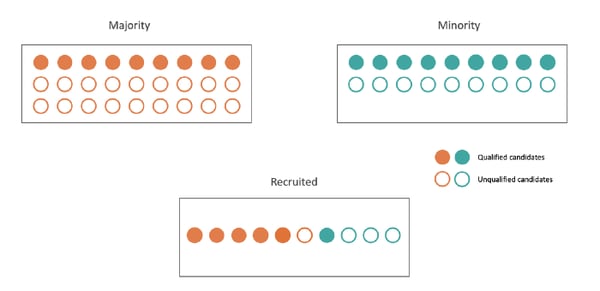
 Demographic parity (with laziness)
Limitations. On the other hand, demographic parity has various flaws. First, it can be used in an inappropriate context, meaning where disproportionality is truly present and independent from a protected attribute, or from a proxy for the protected attribute. In our example use case, enforcing demographic parity would result in discrimination against some qualified candidates, which could be seen as unfair.
This first flaw underlines one of demographic parity’s problems: it concerns only the final outcome of the model but doesn’t focus on equality of treatment. This lack of fair treatment necessity is demographic parity’s second problem, which is called laziness. Nothing would prevent the use of a trained model to select candidates from the majority group, while candidates from the minority group were selected randomly with a coin toss — as long as the number of selected candidates from each group is valid.
A third flaw is due to demographic parity’s independence from the target variable: in the case where the fractions of suitable candidates in both classes are not equal, which is mostly always the case, demographic parity rejects the optimal classifier 𝐶 = 𝑌.
The last flaw is highlighted by Weisskopf: because demographic parity leads to affirmative action, it leads to recurrent criticism. Such criticism can contribute to undermining the reputation of the minority group in the long term.
Equality of Odds, Equality of Opportunity
As demographic parity’s main flaws are all linked to the inequality of treatment it introduces among subpopulations, two research groups came up with similar definitions of fairness which took into account how each group was treated: Equality of Odds and Disparate Mistreatment. We will use the Equality of Odds denomination in this article.
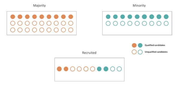
Equality of Odds is defined as the independence of 𝐶 and 𝐴 conditionally on 𝑌. In other words, a classifier treats every subpopulation the same way if it is has the same error rates for each subpopulation.
The mathematical definition of equality of odds is:

However, in the same way that reaching demographic parity is very hard in practice, finding a model that satisfies equality of odds is challenging and often comes at the price of low model performance.
 Equality of Odds. Notice that, in order to satisfy this definition, more than half of the recruited candidates have to be unqualified.
In the same way a relaxed version was defined for demographic parity, Hardt, Price, and Srebro defined equality of opportunity as a weaker version of equality of odds. Equality of opportunity results in applying the equality of odds constraint only for the true positive rate so that each subpopulation has the same opportunity to be granted the positive outcome.
Equality of opportunity is defined as:

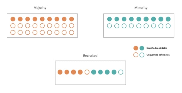
To get back to our recruitment example, satisfying equality of opportunity means that we would recruit the same ratio of qualified candidates from each subpopulation.
 Equality of Opportunity
In practice, as we cited before, equality of odds and equality of opportunity both have the ability to guarantee equality of treatment among subpopulations. Thereby, they also sanction laziness, which was one of the demographic parity definition flaws. This definition also gets rid of the fact that demographic parity was rejecting the optimal classifier 𝐶 = 𝑌. In that case, both false positive and false negative rates would be 0% for the whole population, meaning 0% for each subpopulation, proving that the optimal classifier satisfies both equality of odds and equality of opportunity.
Limitations. However, there are two main flaws linked to equality of odds (and equality of opportunity) and both can be summed up by the fact that this definition might not help deal with unfairness problems in the long term. First, it doesn’t take into consideration possible discrimination outside of the model. As an example, as protected attributes (race, gender, class, etc.) have more or less always had an impact on access to opportunities such as loans or education, such discrimination could result in an unbalanced ratio between the privileged and unprivileged class, which will just be replicated by a model satisfying equality of opportunity.
So, in our recruiting case, if only 10% of our candidates are from the unprivileged class (because the job is highly qualified and only few people from the unprivileged class have had access to higher education), only 10% of the finally recruited candidates will be from the unprivileged class.
The second flaw is a consequence of the first one in the case where there is an extreme difference between the privileged and unprivileged groups. In that case, by preserving the contrast, the model satisfying equality of opportunity might in the long term increase this difference, resulting in a vicious circle.
Predictive Rate Parity
A slightly similar fairness definition is predictive rate parity and was introduced by Dieterich, Mendoza and Brennan.
A model satisfies predictive rate parity if the likelihood of the positive observation of the target variable among people predicted with the positive outcome is independent from the subpopulation.
Mathematically speaking, predictive rate parity is defined as follows:

In practice, relaxed definitions also exist for this definition, and, depending on the value of interest of 𝑌, we can talk about positive predictive parity or negative predictive parity. Positive predictive parity is defined as follows:

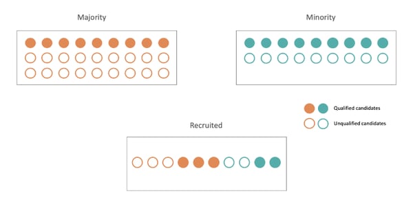
A practical example is that, among all the recruited candidates, the same proportion of really qualified applicants should be the same. Respectively it means that the recruitment errors are spread homogeneously among subpopulations. Thereby, predictive rate parity should guarantee that candidates are chosen by the model based on their real qualification for the job.
 Positive predictive parity. Notice that it isn't possible to satisfy predictive rate parity in this situation.
As the notion is similar to equality of opportunity, one of its advantages in practice is that it validates the optimal classifier 𝐶 = 𝑌, as both necessary probabilities are equal to 1 in the case of perfect classification. Another advantage could be called inclusiveness, as predictive rate parity (and especially positive rate parity) literally means that the chances for a recruited individual to succeed are the same no matter the subpopulation it belongs to.
Limitations. However, this definition’s resemblance with equality of opportunity also makes its flaws similar: it doesn’t take into account unfairness preexisting among candidates and replicates it. Models corrected under predictive rate parity can also boost unfairness in the long term. In practice, this method also has definition flaws: it needs access to the true value of the target, which is sometimes hard to define (true qualification for a job as an example) and it is very similar to equality of opportunity but way more difficult to implement in practice.
No Free Lunch in Fairness
Now that we’ve explored the different types of fairness definitions, we have to highlight a fairness property that has crucial importance when correcting unfair algorithms in practice.
This property is called the Impossibility Theorem of Fairness and states the pairwise incompatibility of all group fairness definitions discussed here (demographic parity, equality of odds, and predictive rate parity).
It is impossible to satisfy all definitions of group fairness, meaning that the data scientists need to choose one to refer to when starting a fairness analysis.
Conclusion
On top of biased data issues (cf. our previous article) lies another obstacle when it comes to correcting unfairness in practice: there is no consensus on the definition of fairness. Already existing legal material is too vague to be used in machine learning, and there are currently six main fairness definitions across research papers on fairness: Unawareness, Demographic Parity, Equality of Odds (and of Opportunity), Predictive Rate Parity, Individual Fairness, and Counterfactual Fairness.
The Impossibility Theorem of Fairness proves that Demographic Parity, Equality of Odds, and Predictive Rate Parity are pairwise incompatible, which makes satisfying all fairness definitions impossible. Therefore, we face a practical dilemma when it comes to designing fair machine learning models — there’s no “best” answer.
Now that we’ve defined how to detect unfairness in machine learning models, the next article in our fairness blog posts series will focus on how to correct unfair models.


