


Data is constantly changing, as the world from which it is collected. When a model is deployed in production, detecting changes and anomalies in new incoming data is key to make sure the predictions obtained are valid and can be safely consumed. So, how do we detect data drift?

In this article you will learn about two techniques used to assess whether dataset drift is occurring: the domain classifier, looking directly at the input features, and the black-box shift detector, indirectly studying the output predictions.
While both techniques work without ground truth labels, the black-box shift detector is cheaper (as it does not require any training) but in some cases less effective as it needs more data to trigger an alert than the domain classifier.
Although they perform similarly in many cases, they are designed to capture different changes and are complementary for specific types of shift, overall covering a wide spectrum of drift types. Let’s see how they work!
The Electricity Dataset
Here we focus on classification tasks and take the electricity dataset as an example, on which we train a classifier, say a random forest, to predict whether the price will go UP or DOWN. We call this classifier the primary model. Now let’s imagine we get a second new electricity dataset. We want to know if there is a substantial difference between the original dataset and the new dataset before scoring it with our primary model.
Brief Recap on Data Drift
What is generally called data drift is a change in the distribution of data used in a predictive task. The distribution of the data used to train a ML model, called the source distribution, is different from the distribution of the new available data, the target distribution.
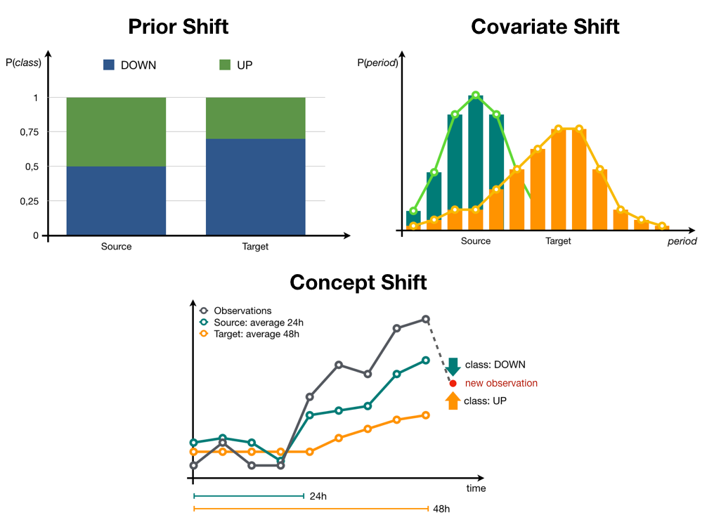
When this change only involves the distribution of the features, it is called covariate shift. One simple example of covariate shift is the addition of random noise to some of the features in the dataset. Another type of data drift is prior shift, occurring where only the distribution of the target variable gets modified, for instance changing the proportion of samples from one class. A combination of the previous shifts is also a possibility, if we are unlucky.
Probably the most challenging type of shift is the concept shift, in which case the dependence of the target on the features evolves over time. If you want to know more about the data drift, have a look at our earlier post, A Primer on Data Drift.
An illustration of the possible types of drifts for the electricity dataset is shown in Figure 1. In this post we’ll focus on covariate and prior shifts, as their detection can be addressed without ground truth labels.
Domain Classifier for Covariate Shift
We can train a binary classifier on the same features used in the primary model to predict which domain each observation belongs to: source or target. This is exactly how we build a domain classifier. If the two datasets are different enough, the domain classifier can easily discriminate between the two domains and exhibits high accuracy, which serves as a symptom of drift. We perform a Binomial test checking how likely is to get such accuracy when there is no drift. If the p-value — i.e., the probability of getting at least such accuracy under the no drift hypothesis — is low enough, this means that a drift might be occurring. In practice, we trigger a drift alert when the p-value of the Binomial test is less than a desired significance level.
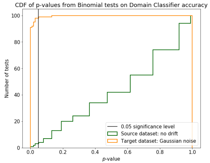
Using the Binomial test on the domain classifier accuracy is more reliable than directly looking at the accuracy itself. Figure 2 shows how the distributions of the p-values change on the source and target dataset, illustrating how effective this tool is to discriminate the two situations.
By design, the domain classifier is meant to detect alterations of the input features (covariate shift)and is not adequate in case of shifts affecting only the label distribution.
This technique requires performing a new training every time that a batch of new incoming data is available. In this sense, the domain classifier is expensive, but it has many advantages. One of its most appealing aspects is that it can be used locally, at the sample level, to predict which observations are the most different from the original dataset. Thus, this simple technique allows a deeper analysis of the drift condition and, in particular, is able to deal with partial drift, a situation when only a part of the observations or a part of the features are drifted.
Black-Box Shift Detector for Prior Shift
What if we can’t afford training a new model every time? Or if we have no access to the features used by the deployed model?
In this case, we can build a shift detector on the top of our primary model. Here, we use the primary model as a black-box predictor and look for changes in the distribution of the predictions as a symptom of drift between the source and target datasets [1].
Unlike the domain classifier, the black-box shift detector is designed to capture alterations in the label distribution (prior shift) and is not adequate in case of covariate shifts that have little impact on the prediction, such as small random noise.
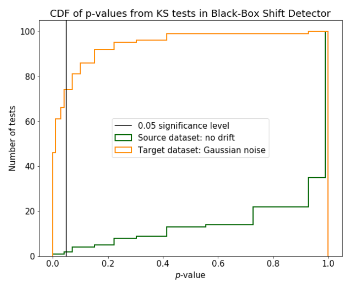
After collecting the predictions of the primary model on both source and target datasets, we need to perform a statistical test to check if there is significant difference between the two distributions of predictions. One possibility is to use the Kolmogorov-Smirnov test and compute again the p-value, i.e., the probability of having at least such distance between the two distributions of predictions in case of absent drift.
For this technique we are looking at the predictions (which are vectors of dimension K), the number of classes, and perform K independent univariate Kolmogorov-Smirnov tests. Then we apply the Bonferroni correction, taking the minimum p-value from all the K tests and requiring this p-value to be less than a desired significance level divided by K. Again we can assume there is a drift when the minimum p-value is less than the scaled desired significance level. Figure 3 shows how the distributions of the p-values change on the source and target datasets.
How can we be sure that only looking at new predictions, one can tell whether the features or the labels distribution has changed? What is the connection between predictions, features and true (unknown) labels?
Under some assumptions, [1] the distribution of the primary model predictions is theoretically shown to be a good surrogate of both features and true unknown labels distributions.
In order to meet the required assumptions to use a black-box shift detector, we first need to have a primary model with decent performance. This one should be easy — hopefully. Second, the source dataset should contain examples from every class, and third we need to be in a situation of prior shift. This one is impossible to know beforehand, as we have no ground-truth labels. Although in real life scenarios it’s impossible to know whether those theoretical hypotheses are met, this technique is still useful in practice.
Shaking the Dataset to Measure Robustness
In order to benchmark the drift detectors in a controlled environment, we synthetically apply different types of shift to the electricity dataset:
- Prior shift: Change the fraction of samples belonging to a class (technically this could also change the feature distribution, thus it is not a ‘pure’ prior shift).
- Covariate Resampling shift: Could be either under-sampling or over-sampling. The former case consists in a different selection of samples according to the features values, for instance keeping 20% of observations measured in the morning. The latter consists in adding artificial samples by interpolation of existing observations.
- Covariate Gaussian noise shift: Add Gaussian noise to some features of a fraction of samples.
- Covariate Adversarial shift: Amore subtle kind of noise, slightly changing the features but inducing the primary model to switch its predicted class. This type of drift is less likely to occur and difficult to detect, but its negative impact is large.
Prior and Covariate Resampling shifts are the most common in a real-world scenario because of the possible selection bias during data collection.
In the experiments, we use 28 different types of shifts from these four broad categories, as detailed in the following table for the curious readers:
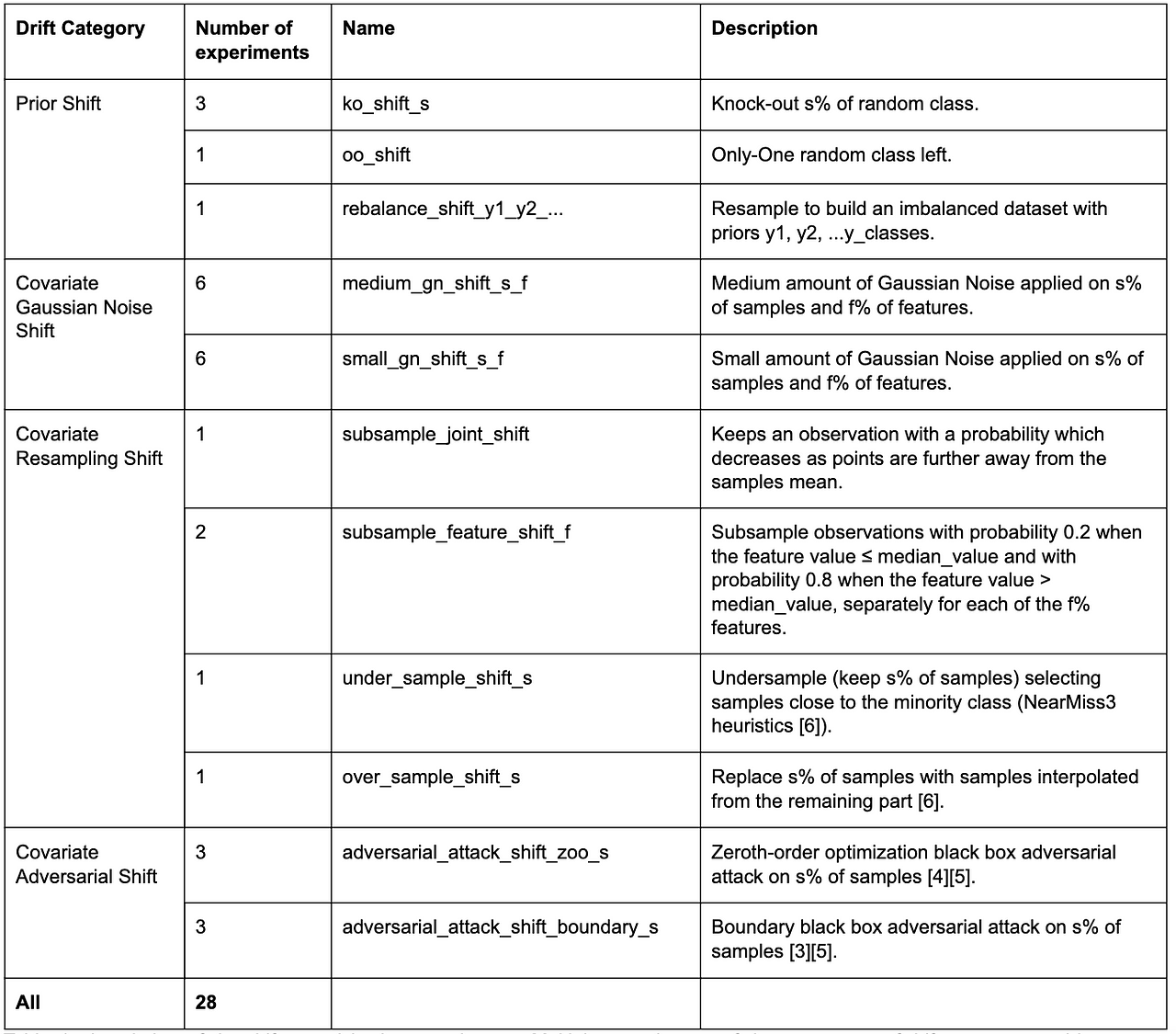
For the experiments and to generate a part of the shifts, we use the library provided in the Failing Loudly github repo [2]. For the adversarial shifts, we use the Adversarial Robustness Toolbox [5], while for some of the resampling techniques, we use imbalanced-learn [6].
Benchmarking the Drift Detectors
An ideal drift detector is not only capable of detecting when drift is occurring but is able to do so with only a small amount of new observations. This is essential for the drift alert to be triggered as soon as possible. We want to evaluate both accuracy and efficiency.
We apply 28 different types of shifts to the electricity target dataset from the four categories highlighted in the previous section. For each shift situation, we perform 5 runs of drift detection by both domain classifier and black-box dhift detector. For each run, we perform the detection comparing subsampled versions of the source and drifted datasets at six different sizes: 10, 100, 500, 1000, 5000, and 10000 observations.
Both the primary model underlying the black-box shift detector and the domain classifier are random forests with scikit-learn default hyper-parameters.
An example of the detection results obtained for a set of covariate resampling shifts is shown in Figure 4. The lines show the average p-values across the runs, while the error areas show the standard deviation of the p-values. The more samples available, the higher the chances to detect the drift.
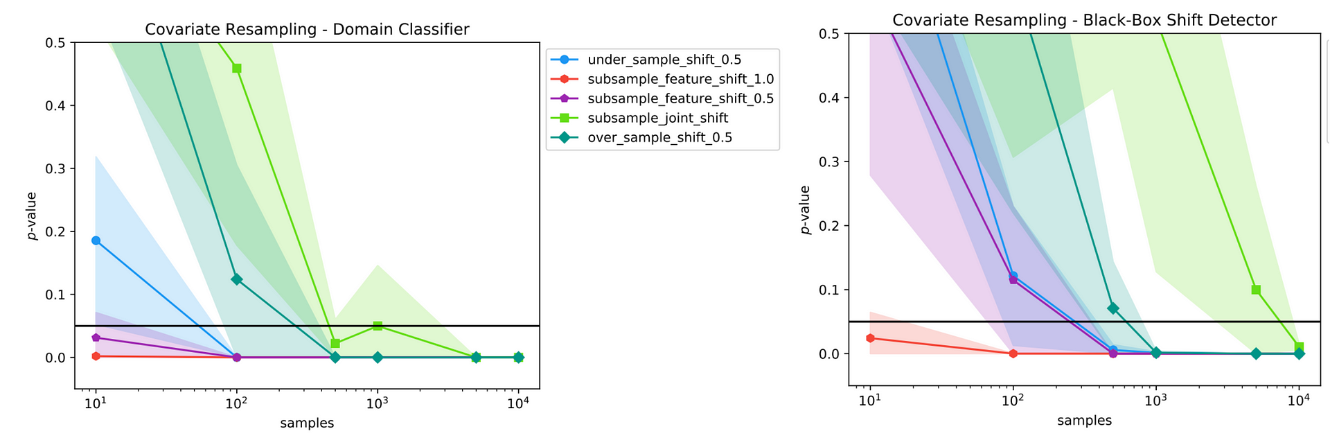
Some of the drifts will cause the primary model to vastly underperform with a large accuracy drop. Although in a real scenario it would be impossible to compute this accuracy drop without ground truth labels, we highlight this information to better illustrate the different types of shift. The drifts yielding to high accuracy drop are the most harmful for our model. Still, whatever alteration may affect the accuracy, it is important to be aware that some change is occurring in the new data and we should probably deal with it.
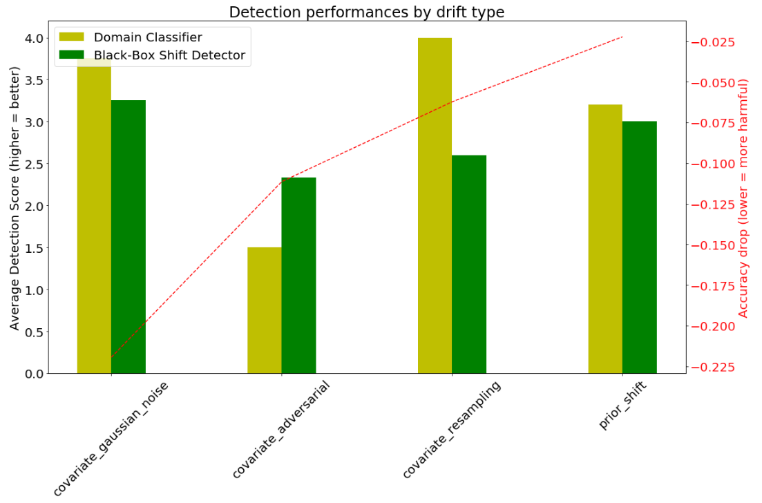
In order to measure the efficiency of the drift detectors, we score the two techniques with respect to the minimum dataset size required to detect a particular drift. We assign a score from 6 to 1 if the detector first detects a drift at dataset size from 10 to 10000; the detector gets 0 score if it can’t detect the drift at all.
The results obtained for the black-box shift detector and the domain classifier are averaged by type of drift and shown in Figure 5 alongside with the average accuracy drop.
Who’s the Best Drift Detector ?
We can see that the two methods perform similarly in case of Gaussian noise shift. The adversarial noise is so subtle that the Domain Classifier has some trouble catching changes in the features. On the other hand, as the adversarial noise is designed to make the predictions change, it does not go unnoticed to the black-box shift detector, which is more efficient in this case. The prior and covariate resampling shifts are less harmful to the primary model for this dataset, which also makes the black-box shift detector miss some of them, revealing the domain classifier as more efficient for the most frequent real-world types of shift.
Takeaways
Domain classifier and black-box shift detector are two techniques looking for changes in the data, either directly looking at the features or indirectly at the model predictions.
They perform similarly on many different situations of drift, but there is a divergence in two situations: the domain classifier is more efficient in detecting covariate resampling drift (the most common case of dataset shift) while the black-box shift detector is more efficient in catching adversarial noise.
The black-box shift detector is the way to go if the features are not available and the primary model in production is indeed a black-box, but high model performance might be a hard requirement for some specific types of drift.
The domain classifier has also a great advantage of being able to score individual samples, thus providing a tool to perform a deeper local analysis and identify possible anomalies.
References
[1] Z. C. Lipton et al. “Detecting and Correcting for Label Shift with Black Box Predictors”, ICML 2018.
[2] S. Rabanser et al. “Failing Loudly: An Empirical Study of Methods for Detecting Dataset Shift”, NeurIPS 2019, and its github repo.
[3] PY. Chen et al. “ZOO: Zeroth Order Optimization Based Black-box Attacks to Deep Neural Networks without Training Substitute Models”, ACM Workshop on Artificial Intelligence and Security, 2017.
[4] W. Brendel et al. “Decision-based Adversarial attacks: reliable attacks against black-box machine learning models”, ICLR 2018.
[5] Adversarial Robustness Toolbox: IBM toolbox to generate adversarial attacks.
[6] imbalanced-learn: library with resampling techniques for imbalanced datasets.