


Financial instruments like options and futures have been around for quite a while, and although they became quite notorious during the 2008 stock market turmoil, they serve a real economic purpose for lots of companies around the world. Before getting into the details on how to use machine learning for option pricing (and more specifically deep learning), we’ll take a step back to understand the purpose of options via a concrete example.

About the Author: Alexandre Hubert began his career as a trader in the city of London, and shifted to become a data scientist after four years. He has worked on a wide range of use cases, from creating models that predict fraud to building specific recommendation systems. Alex has also worked on loan delinquency for leasing and refactoring institutions as well as marketing use cases for retailer bankers. Alex is a lead data scientist at Dataiku, located in Singapore.

Options 101
Why are they important?
Let’s say we are a biscuit manufacturer and our mission is to bring to our customers the best possible biscuit with a consistent level of quality and a very stable price.
To produce these delicious biscuits our factories need lots of wheat, which the company buys on a monthly basis. However, the price of wheat is dependent on lots of different factors, which are hard to predict or control. For example, if the weather is poor in a large producing country, the market will face a shortage in supply resulting in the wheat prices going up.

Unfortunately, there’s no way we can know six months in advance what the weather will be. And that price needs to be as predictable as possible, as our beloved customers will expect the same quality for their favorite biscuits at a consistent price for years to come.
As a biscuit manufacturer, we would therefore really appreciate having the right to buy a certain quantity of wheat at a certain price on a certain date. In our example, that would mean buying 30T of wheat in six months at $100 per pound (in practice things are more standardized, but we want to keep things simple).
It’s worth noting that this right is not an obligation to buy the wheat, the real advantage being if the price of wheat is much lower than $100/lb in six months, we aren’t obligated to buy it at the higher price.
However, if because of global warming and an incredibly hot summer throughout Europe the harvest was not good and a shortage in supply drove prices up above $150 USD/lb , that right to buy at $100 will become very handy and will result in savings of $50/lb.
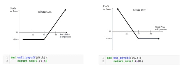
That right to buy or sell an asset at a given price at a certain date is called an option contract. The right to buy is better known as a call contract and the right to sell is known as a put contract. Here is its payoff at expiration — also important for the rest of the story.
How are options used?
Options are available as financial derivatives listed on the financial markets and are very often quoted by financial institutions. Therefore, to find the right to buy 30T of wheat in 6 months at $100 , it is very likely that the CFO of our company will call a couple of bankers and ask them to provide a quote.
This has a huge implication on the bankers side. They compete against one another, and it is important for them to have the right estimation of the fair price. As a matter of fact, if Bank A is quoting $10/lb but bank B quotes $9/lb, most CFOs (being rational and conscious with the money of the company) will choose to do business with Bank B, which will imply a loss in revenue for Bank B.
And at the same time, neither of the banks can offer a price too low to win the bid. As a matter of fact, although it is an intangible service that they provide, it has a minimal cost that cannot be ignored. Going below a certain threshold would imply a misuse of capital and could potentially attract the terrible arbitrageurs (I won't go into the details of what arbitrage is — you can find lots of interesting resources here), which would also mean a loss in revenue at the end for the bank.
Thus, the bank must have a correct appreciation of what the fair price is to avoid losing money because of the arbitrageurs and still offer a better price than its competition. The question is then — how do we price an option?
How are they priced?
In 1973, Black and Scholes came up with a formula to price an option (they revisited it slightly and got offered a Nobel Price in 1997).
Now that we are comfortable with what the payoff of an option will look like at the expiration depending on the price of the underlying asset — go back and look at the payoffs charts until it makes sense — we can have an inkling of what we need.
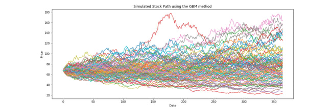
If we had a method that let us simulate (that is, generate enough of the possible or realistic trajectories for the price of wheat in the next six months), we could then use the payoffs formula to have a fair estimation of the option price. The key thing is to be sure that the generated price paths are realistic and mimicking the price of wheat for the next six months.
As a matter of fact, if the generated distributions of prices at expiration does not match the empirical distributions, our pricing method will be useless. That is called a monte carlo pricing method, and for it, we need:
-
A generic stochastic model that helps generate a great number of possible path prices for wheat for the next six months, matching the empirical log returns distributions.
-
To compute the payoff of our option for each of those path prices.
-
To create an average of the generated payoffs and imply a fair price.
Easy enough!
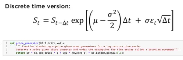
Which model should we take? Black, Scholes, and Merton studied the stock market prices and came to the conclusion that the log return of the prices would follow the hypothesis of stationarity (using some work from Louis Bachelier in 1900 - théorie de la spéculation).
And this was super helpful, as that hypothesis would therefore imply that the price of wheat would follow a Geometric Brownian Motion that could be synthesised with a very elegant equation using the normal distribution.
That all sounds great. Why are we talking about GANs then?
There is just one slight problem with this approach: it's wrong. Doing machine learning, we all try to optimize a cost function and are prone to accept a certain degree of error depending on the complexity of the problem and the cost of error. However, it is terribly wrong:
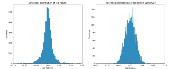
A quick comparison of the empirical distribution of stock return against the stock generated by the normal assumption shows that the reality is not properly captured by the model. In particular, the tail of the curve that represents huge periods of stress (heavy negative return) or euphoria (super positive return) are not captured properly (some arbitrageurs — like Nassim Taled — have benefited greatly from this, as described in the book Le Fric).
Those models are still in place. Well, not exactly those ones — they have been improved slightly to try and better capture reality (ARIMA/ARCH/GARCH, etc). But they remain heavy parametric models under the assumption of stationarity of the log returns.
To improve that modelization significantly and make sure that we price our options better, it would be very nice to have a modelization technique that does not rely so much on such a hypothesis. In the best possible world, it would not rely on any assumption at all. This is where GANs come into play.
Gans 101
What the hell is a GAN?
GANS garnered lots of attention as soon as the original paper by Goodfellow in 2014 got published. They proved their ability to generate images realistic enough so that a human eye would not be able to tell which example is true and which one had been generated. Years later, the improvements are mind blowing, yet the bad publicity of some fake examples taken as real ones started to raise a dark side of GANs.
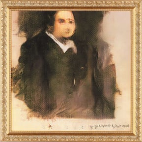
AI art that sold at Christie's (Image Source)
On a brighter note, they became so good at generating that a piece of modern art completely generated by a Network has been sold at Christies for about £300k.
How do they work exactly?
The architecture of GANs is quite elegant.
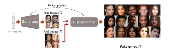
A generator is in charge of creating an image out of pure noise. Just imagine yourself sitting at your desk in a figurative art class, taking a pencil and drawing something with it completely randomly. As one would guess, the first try would not particularly impress your instructor, who would then give you some instructions to improve. Your instructor is what is called the discriminator in the GAN architecture. It is in charge of recognizing real examples from generated examples.
It is those adversarial forces involved in a zero sum game, one trying to generate something as real as possible while the other trying to recognize the real from the generated, that makes the GANs so powerful at generating real examples (it also gives them their name: Generative Adversarial Networks).
How can they be useful in our use case?
With that in mind, if we could have a generator that was trained to draw as realistic log returns distributions as possible, that would be great. We could then see a significant improvement from the normal distribution assumption and be able to build a better pricer for our model.
Therefore, our goal is to train a generator that would create a time series of 50 (arbitrary number) points. Its work would then be submitted to a discriminator in charge of recognizing real stock path trajectories coming from the S&P 500 and those generated by our generator.
That GAN would generate a very high number of possible stock paths, so we would then compute all the possible pay-offs of our options and average them to have the fair price of the options.
How are our GAN(s) actually built?
At this stage, everyone with a little bit of experience in financial markets would argue that each asset has a very specific signature, captured via concepts like the volatility of the trend, which make each distribution unique. It is therefore very unlikely we’d find one model that would generalize to all of the different tickers we are considering.
To overcome that issue, we will train one GAN per ticker from the S&P 500. To do so, we trained our discriminator by using daily data from the S&P 500 tickers between 2002 and 2017. That represents about 4,500 daily stock prices. Out of that, we created roughly (4,500 - 50) time series per ticker by simply rolling from day 0 to day 4450.
We chose a very simple architecture to demonstrate the value of this use case - iterative data science and pragmatic deep learning should start with some quick wins before refining the work and optimizing the models.
We therefore just stacked some Dense layers and used that very informative GitHub repository to avoid common pitfalls during the training to make sure our model would converge.
Results
That sounds all great, but did we get the quick win?
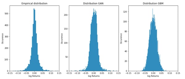
A quick overview of the different results prove at one glance that the GAN does a better job at capturing the empirical shape of a given ticker than the assumption of stationarity of the log returns. It captures the rare events much better as well as the period of calm on the market.
Although this is a significant improvement over a traditional method, there are a couple of things to consider:
- First and foremost, one key trap to avoid in data science is bias. By working on the listed 500 tickers in the S&P 500, we are prone to survival bias that makes us only consider the stocks that survived the darkest hours of 2002 and 2008.
That means that none of our GANs are trained to generate extremely rare events that could potentially result in the delisting of a stock or worse, its filing for bankruptcy.
When data scientists, quants, and machine learning researchers are working on ways to model the real world, it is their responsibility to make sure that the models minimize bias as much as possible or at least make them clear to the audience likely to use the model.
- Second of all, now that we managed to demonstrate some quick wins, it's important to improve the model — the use of LSTM or attention models in the generator and discriminator shows some significant improvements in the way GANs capture the empirical distribution. But it's also a very good time to start to productionalize this use case. It stays sterile if it is just available on my Jupyter notebook.
From my experience in the front office, I would need to deploy those models behind a REST API that would serve the desk and help the traders/structurers etc to make more accurate pricing.
BONUS: You enjoyed this tutorial on using machine learning for option pricing? Why not do it all with Dataiku? Download the free edition to give it a try.
Disclaimer: This is not an article that aims at giving methods to invest on the financial markets. If you were to reuse some ideas taken out of the article, they should be done at your own risk and not the expense of the author nor the company he works for.