


“The essence of abstractions is preserving information that is relevant in a given context, and forgetting information that is irrelevant in that context.” -John V. Guttag
Given the maturity that machine learning is reaching, it becomes increasingly important to follow standardization and extension principles specific to software engineering. Undoubtedly one of the most used libraries in the field of machine learning is scikit-learn. The tool offers an abstraction called Pipeline, through which it is possible to rationalize the flow of machine learning transformations in order to write code ready for production and to be easily reused.
Advantages
The transition from unstructured code to the use of pipelines brings numerous advantages:
1. Both the transformations of the dataset and the configurations of the models are expressed
Experiment: For example, if you want to perform a grid search also on data transformations, such as the standardization of one variable, this can be easily carried out.
Shift to production: For example, a PCA step before the model estimation becomes part of the pipeline. That pipeline can be shared between experiment and production.
2. Rapid transition into production (even with complex preparations)
The pipeline used to train the model can be reused to make the prediction in production.
3. Increased efficiency and thus, economies of scale
It makes the code much easier to reuse among different analyses or projects.
4. Helps standardize analysis production processes
In enterprise environments, it is important to follow standards to reduce errors and improve understanding of the code.
5. Wide community support
Use of quality libraries, maintained over time and supported by the community.
Scikit-Learn’s Basic Elements
Transformer
Transformer takes a set of input data, applies a transformation to it, and returns the modified data to the output. These classes must implement the transform method and encapsulate a set of data transformation logics. There are several Transformer defaults from the scikit-learn library, but new ones can be also created.
Predictor
Through the Predictor class, it’s possible to train a model based on a certain training set (potentially pre-processed through Transformer) and use it on fresh data. These classes must implement the predict method. Scikit-learn gives you a possibility to create a custom Predictor which can be, for example, a classifier or a regressor.
Pipeline
This object allows you to chain multiple transformations followed by a final Predictor. This describes the transformation logics and the configuration used in the model used for the prediction.It is important to note that a pipeline can be composed by other pipelines.
Scikit-Learn’s Advanced Elements
FeatureUnion
Through this element, it is possible to create multiple Transformers that start from the same input and produce independent outputs. The result of each Transformer is then added to the final DataFrame.
ColumnTransformer
Through the Column Transformer, it is possible to carry out different transformations that start from the same DataFrame but perform different transformations on different sets of columns.
Create Your Own Transformer or Predictor
Sometimes, especially in an enterprise project, it is necessary to create our own Transformer or Predictor. Although not explained in this article, scikit-learn allows you the possibility to do this. However, you can see an example below where an extended version of XGBoost is used to implement ‘early stopping’ to prevent model overfitting.
Example
An example of a Pipeline which carries out different transformations (imputation of missing values, vectorization, PCA, etc.) is provided below.
from sklearn.compose import ColumnTransformer
from sklearn.pipeline import Pipeline,FeatureUnion
from sklearn.feature_extraction.text import CountVectorizer
from sklearn.decomposition import PCA, TruncatedSVD
from xgboost import XGBRegressor
from sklearn.impute import SimpleImputer, MissingIndicator
from sklearn.preprocessing import OneHotEncoder
import sklearn

sklearn.set_config(display="diagram")

discrete_transformer = Pipeline(
steps=[
('imputer', SimpleImputer(strategy='median'))
])
categorical_transformer = Pipeline(
steps=[
('imputer', SimpleImputer(strategy="constant",fill_value="missing")),
('ohe', OneHotEncoder())
])
text_transformer = Pipeline(
steps=[
('cv', CountVectorizer(analyzer="word",ngram_range=(1, 1), max_features=2000) ),
('pca', TruncatedSVD(n_components=100))
])
pre_processing = ColumnTransformer(
transformers=[
('discrete', discrete_transformer, ['points']),
('categorical', categorical_transformer, ['country']),
('text', text_transformer, 'description')
])

final_pipeline = Pipeline(
steps=[
('feature_engineering', FeatureUnion([
('type_specific', pre_processing),
('missing_flag', Pipeline([
("missing_indicator", MissingIndicator(error_on_new=False)),
("pca", PCA(1))
]))
])),
('regression', XGBoostRegressorWithEarlyStop())])

final_pipeline.fit(X_train,y_train
This code aims to demonstrate how the organization in Pipeline leads to writing more compact and understandable experiment codes.
Furthermore, using a new scikit-learn feature, it is possible to graphically show the pipeline’s DAG (Direct Acyclic Graph). To enable it, the code below is used:
sklearn.set_config(display="diagram")
The diagram below offers a high-level view of the whole experiment to aid understanding.
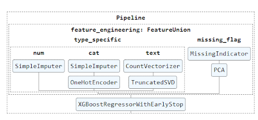
It is important to note that ‘XGBoostRegressorWithEarlyStop’ is a custom Predictor which results from the extension of the base XGBoostRegressor (xgboost library) estimator where the early stopping feature was included.
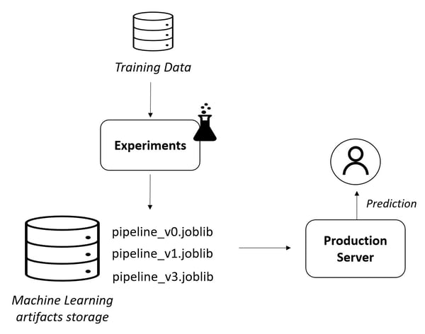
Speaking of transition to production, the use of pipelines allows you to save not only the developed model but also all the transformations made on the variables. To persist the pipeline we can use the joblib library. A good practice is to store all the developed pipelines, versioning them in a dedicated storage location. Here is an example of code to store the pipeline:
# LAB
import joblib
# Export the classifier to a file
joblib.dump(final_pipeline, 'model.joblib')
For the production environment, you can simply load the previously saved pipeline and use it for prediction without worrying about the data preparation.
# PROD
import joblib

new_pipeline = joblib.load('model.joblib')
prediction = new_pipeline.predict(data)
Here an example of a basic architecture that leverages the use of pipeline:
Conclusion
Through the use of pipelines, especially in an enterprise environment, we have several advantages in organizing, maintaining, reusing, and productionizing the machine learning pipeline.
It is especially possible to make changes during experiments without worrying about having to replicate it in production, making the shift to production a seamless process throughout the development phase. Pipelines prove to be a highly valuable tool for the lifecycle of the model, quickly bringing tangible results to data science projects.
The above post is a guest contribution from our friends at BitBang. BitBang is a leader in digital analytics, web measurement consulting, and customer experience management, accelerating business transformation through data strategy and data execution practices.