


Many millennials in the United States are burdened with high student loan debt. Outstanding student loan debt in the United States was at a massive $1.19 trillion as of June 2015.
There is a lot of discussion among politicians and the public about what to do about this crippling amount of debt placed upon many Americans. To that end, I wanted to look at how this debt is distributed geographically in the US, and whether communities with a large proportion of debtors are structurally different from other communities.

Investigating Student Loan Debt By Merging Multiple Data Sources
I recently joined Dataiku as a Data Scientist based in New York City. I've spent a lot of time analyzing geospatial data, and I was excited to test the abilities of Dataiku Data Science Studio (DSS) in this realm. While deciding which project I wanted to work through while familiarizing myself with Dataiku Data Science Studio (DSS), I remembered reading about a recently released Internal Revenue Service dataset.
This is a pretty neat dataset. It contains aggregated information at the ZIP code level for all the tax returns collected in the United States in 2014.
My goal for this analysis was to investigate the factors most prevalent in ZIP codes where a high proportion of people were burdened by student loan debt. I also had a few sub-goals:
- Build a heatmap that showed Student Loan debt across the US.
- Learn how to incorporate outside datasets into a model in Dataiku DSS.
- Construct an accurate regression model to predict the proportion of student loan debt in a given ZIP code.
Internal Revenue Service Data (IRS)
My first step was obtaining the IRS dataset from the link above. It contains information from tax returns aggregated by ZIP code. There are 114 variables and around 27,000 rows. (There are many more than 27,000 zipcodes in the United States, but the IRS does not return information on zipcodes with fewer than 100 tax-filers, for privacy purposes.) The variables range from basic information about the number of total returns to counts of every possible deferment and deduction within each zipcode. Since people paying student loans get a tax deduction, we can use the student loan deduction variable as a proxy for the proportion of tax-payers in each zipcode who paid student loans.
A nice thing about using tax information for tracking student loans is that the deduction only counts if the loan is being paid down. Since student loans do not require payment until after a tax-payer leaves school, the dataset naturally ignores current students.
In Dataiku DSS I can create a histogram of Zipcode population (or any other numeric variable) with a single click. I see that it decays exponentially, with a median at 2,060:
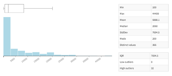
Histogram of Population of Zipcodes
Since my inital dataset was all raw counts, the variable I was trying to predict does not exist yet. To create it, I simply add a formula during the cleaning portion of my flow.
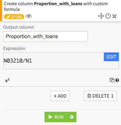
Creating a proportion column in Dataiku DSS
After I create the new proportion variable "proportionwithloans", I can look at the histogram for my new data. It looks close to normally distributed, with a bit of a right skew. However we immediately notice that there are a lot of 0 values. We will have to find a way to deal with them later.
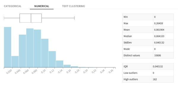
Histogram of Proportion with Student Loans in Zipcodes
Census Data
Whenever I am trying to build a model for a dataset, I always like to ask some of my non-Data Scientist friends what would best predict my outcome variable.
In this case, I heard the same answer several times: "The proportion of people with student loans in a ZIP code should be predicted by the age of the people in that ZIP code." This seemed pretty rational to me, so I knew I had to get demographic data by ZIP code.
Happily, Nicolas Gakrelidz, a Senior Data Scientist at Dataiku has been compiling and cleaning a detailed set of US Census and American Community Survey data for Dataikers to use. (The dataset can also be made available to our clients - just email Nicolas).
The census dataset has a LOT of information. It has thousands of variables dating from the 2010 US census, all aggregated by ZIP code. After some cleaning and limiting the variables to those that had to with age, I was able to merge the Census data set with the IRS dataset, all within Dataiku DSS. The only code that I had to write during these steps was a little bit of Python to turn all of the raw counts into proportions in both data sets.
# Pattern of numeric variables
pattern   = re.compile('[A-Z]\d{5}')
col_names = [col for col in
             zip_data_no_global_df.columns if pattern.match(col)]
col_names.extend(['MARS1','MARS2','MARS4','PREP','N2','NUMDEP'])

# divide numeric columns by population
for col in col_names:
zip_data_no_global_df[col] = zip_data_no_global_df[col] /
                               zip_data_no_global_df.N1
Visualizing Student Loans
Before building my model, I wanted to construct a map of the way student loans were distributed across the country. I did this by downloading two plugins:
- the Reverse geocoding Dataiku DSS plugin, which opens up access to the built-in mapping features of Dataiku DSS.
- the Zipcode geocoding plugin, which allows me to get a lat and lon at the center of each ZIP code, which in turn will let me aggregate the ZIP codes into counties.
Here is what a zipcode-level map of the United States looks like:
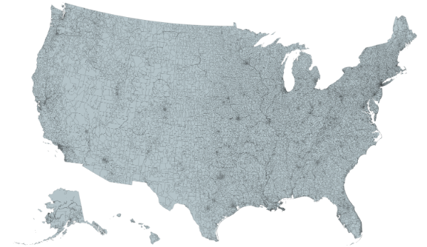
Map of US zipcodes
The bins on the zipcodes are so small that it's just a lot easier to see the population distributions when they are aggregated to counties. Building the map aggregated to counties was as easy as geocoding my latitude and longitude using the built-in geocoder, then selecting the Filled Administrative Map chart from Dataiku DSS's charts section.
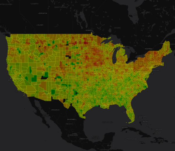
Heatmap of Proportion with Student Loans by County
Student loans seem to a bigger problem in the northern US than the southern US, and to be an especially large issue in New England and the Breadbasket. (A fun future project might be correlating the number of Liberal Arts colleges per ZIP with the student loan debt proportion in each ZIP.) Here we can see the area around Burlington, Vermont, which has one of the highest proportions of student loan debtors in the country. Sixteen percent of taxpayers in Chittenden Count, which surrounds Burlington, are paying down student loans.
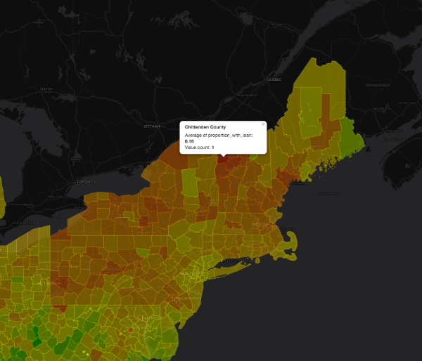
Close up Heatmap of Proportion with Student Loans
Feature and Algorithm Selection
This project was never meant to create a predictor for live data. Instead it is an attempt to investigate possible correlations in an already existing dataset. Because of that, some algorithms that may have the most predictive power but aren't very good at explaining relationships - Random Forest for example - are of limited value. Instead we will look at the lasso regression method. These will tell us not just which features are most important, but which way the features drive our dependent variable.
For feature selection, I allow in all features that do not clearly correlate with student loans. This means removing any tax information that involves education, or even counts of total deductions, since student loans necessarily count among those deductions.
Additionally, I remove all references to geographic location. The map already provides an excellent summary of where in the US people with student loans are living - I'd rather learn which other factors come in to play.
Finally, there is the matter of the large number of ZIP codes that ostensibly have zero people who took the student loan deduction. To avoid having these ZIP codes warp our model, I will build a secondary model to investigate if there are common features among them that strongly correlate with no student loan deductions.
After training this simple Logistic Regression with just a couple clicks in Dataiku DSS, I see that population alone accounts for a very large part of whether a ZIP has zero student loan deductions (in our decision matrix below, true values have at least one loan deduction and false values have none):
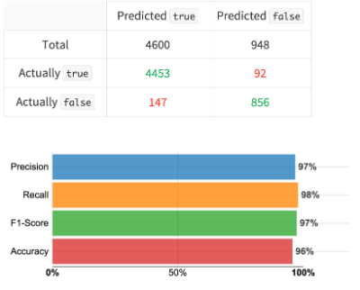
Confusion Matrix for predicting existence of Student Loan Debt in a Zipcode
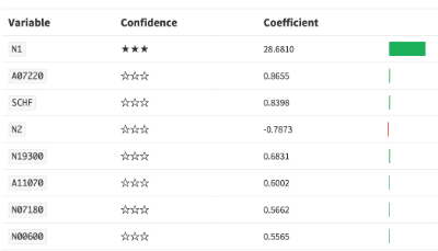
Variable importance for Logistic Regression model. 'N1' is the Zipcode's population
If we filter our dataset to ZIP codes with a population of 500 or greater we can drop nearly all of the ZIP codes with zero deductions and nearly none of the others.
Now that we have our data prepared, and our models selected, we can train our regression models. To reiterate: the goal is to accurately predict the proportion of tax-filers in a zip code that utilized the student loan deduction on their 2013 tax returns.
Results
Using only the built-in features of Dataiku DSS we can easily train a model that returns an R2 value of .73. Lasso regression works well, both as a predictor and for providing a set of features that correlate with our student loan deductions.
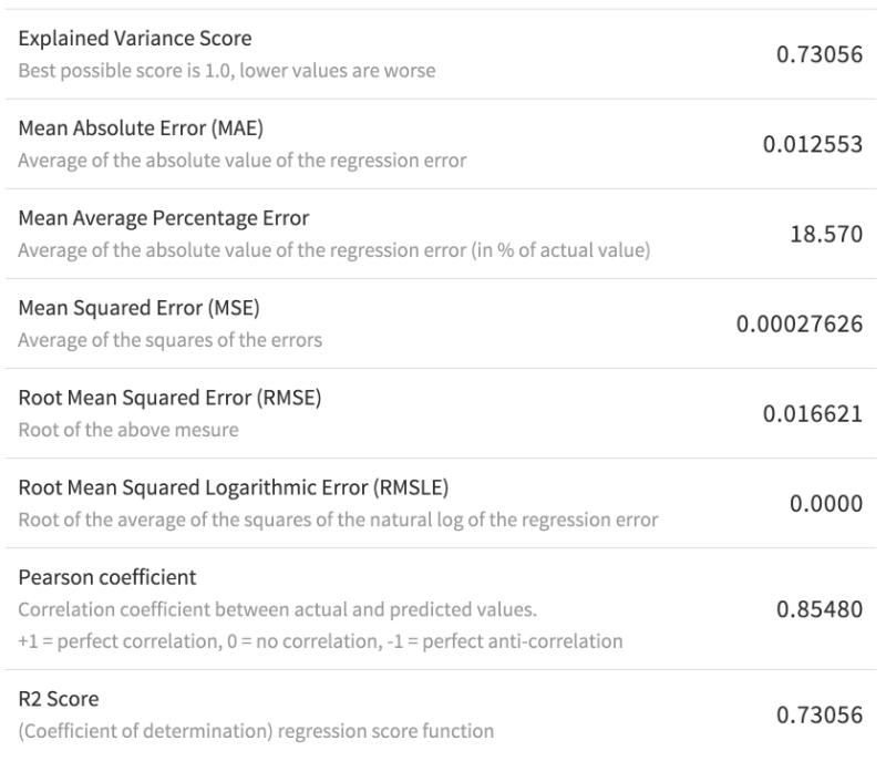
Detailed output of the Lasso Regression model on the test set
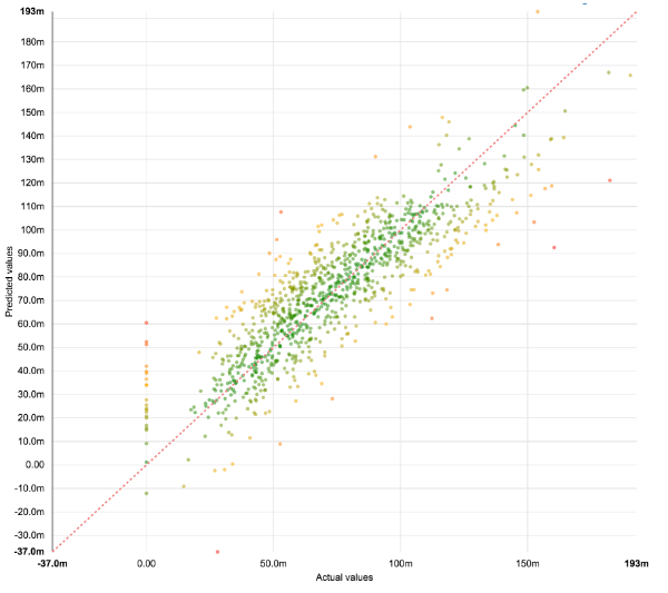
Scatterplot output of the Lasso Regression model on the test set
Of the top six predictive variables, 3 were administrative variables about which tax forms were used and 3 involved filing singly (positive coefficient), or taking child tax credits (negative coefficient).
- A person files singly if they are not married and have no dependents.
- A person can take child tax credits for each child they have as a dependent.
While none of the variables in census dataset were highly predictive, including them did increase the R2 value by .05. It also means that our above variables were the most predictive even when accounting for age of the people in each ZIP code.
Conclusion
The results correlate with a narrative that is often told, but rarely corroborated with evidence.
That is: communities in which a large proportion of the population has student loan debt are less likely to have a high number of people starting families and having children - even when accounting for age. With this data, one could argue that a possible reason for the American trend in having children later could be a result of people's unwillingness to start a family while still mired in massive amounts of student loan debt.
Future Steps
Further feature pruning could increase the p-values of the top predictive variables into a statistically significant range. The addition of datasets such as the aforementioned Liberal Arts college locations could be a good predictor of the geospatial location of the higher areas.
Any questions? Get in touch!