The encoder-decoder framework is undoubtedly one of the most popular concepts in deep learning. Widely used to solve sophisticated tasks such as machine translation, image captioning, and text summarization, it has led to great breakthroughs.
However, when it comes to time series forecasting, the encoder-decoder framework has generated less noise. And yet, the recently emerged models that rely on this architecture have led to more accurate forecasts than classic approaches. They have also proven to be a more scalable solution from a business perspective.
Among them, two have stood out for their performance and scalability: the Multi-Quantile Recurrent Forecaster that comes in two flavors (MQ-RNN and MQ-CNN) and Transformers. Although they both share the same overall architecture, they rely on completely different approaches. Let’s deep dive into their mechanisms!
Objective
The goal of this article is to expose the key principles of these models.
It is the continuation of a two-part series (here’s part one) that aims to provide a comprehensive overview of the state-of-the-art deep learning models for time series forecasting. After reading this series, you will understand:
- What are the key common concepts of deep learning models used for time series forecasting?
- How do these models differ from one another?
- To what extent do they provide better results in terms of forecasting accuracy and computing time?
As an illustrative use case, I will rely on the example of the prediction of daily stock market prices of several companies from different industries over a time window of 30 days. This will provide an opportunity to evaluate and compare the performance of the approaches exposed in two articles on a concrete use case based on different criteria.
1. Deep Learning Models
1.1. Multi-Quantile Recurrent Forecaster (MQ-RNN & MQ-CNN)
Multi-Quantile Forecasters (MQ Forecasters) rely on a Seq2Seq architecture with Context, also referred to as Seq2SeqC, with some slight differences. Let’s first start by describing the Seq2SeqC architecture before diving into the model’s specificities.
What Is a Seq2SeqC Architecture?
Figure 1 illustrates the Seq2SeqC architecture as introduced in [1]. It consists of three major components: an encoder, an intermediate vector, and a decoder.
![Figure 1 — Seq2Seq architecture with Context (Seq2SeqC) as proposed by [1], adapted from [2], illustration by Lina Faik](https://blog.dataiku.com/hs-fs/hubfs/dftt-1.png?width=1000&name=dftt-1.png)
Figure 1 — Seq2Seq architecture with Context (Seq2SeqC) as proposed by [1], adapted from [2], illustration by Lina Faik
Both the encoder and decoder, parameterized by θ, are trained jointly to optimize the log-likelihood computed over the time horizon.
This approach is very similar to DeepAR whose encoder and decoder have the same architecture and share the same weights. More information about this model is provided here.
How Do MQ Forecasters Differ?
Although MQ Forecasters’ architecture is very similar to Seq2SeqC, it differs from it on multiple levels: the loss function, the training scheme, and the neural networks used in the decoder.
Figure 2 summarizes the architecture of MQ-RNN that will be explained in this section.
![Figure 2 — MQ-RNN adapted from [2], illustration by Lina Faik](https://blog.dataiku.com/hs-fs/hubfs/dftt2-Dec-15-2021-08-57-39-09-PM.png?width=1000&name=dftt2-Dec-15-2021-08-57-39-09-PM.png)
Quantile Loss Function:

The quantile loss function allows the weight associated with over-predictions to be varied compared to under-predictions. What does it mean? Let’s suppose q>0.5. The loss has a higher value if the model over-predicts then if it under-predicts.The use of a quantile loss has two main benefits. First, it helps assess the uncertainty of the model predictions, as quantiles can provide an upper and lower bound for forecasts. Second, it makes possible to take into account a difference in costs between under- and over-prediction. For instance, in the retail industry, overestimating the demand leads to storage costs, while underestimating the demand is associated to the lost sale opportunity.
In this context, the model is trained to minimize the total loss which is computed over all time horizons including all quantiles:

What does the quantile loss bring compared to the other approach? This approach has two main advantages:
- It doesn’t make any assumptions on the distributions. There is no need to suppose a certain distribution p(y|θ) for which the model learns to find the parameters θ.
- It produces accurate probabilistic forecasts with prediction intervals. This allows us to know how confident the model is of its predictions and assess the risk associated with them.
Training Scheme
During training, the time sequence is forked. This means that there is a decoder that corresponds to each recurrent layer (time point) and they all share the same weights.
Therefore, at each time point, the loss is computed using the multi-horizon forecasts and the corresponding targets. Then, one back-propagation-through-time gathers the multi-horizon error gradients of different time points in only one pass over the sample.
Thanks to this framework, the model is able to learn more efficiently by using all information in one shot. This allows for a reduction of the training time and a stabilization of the learning as well as a boost in the performance.
Decoder Architecture
Instead of using a Long Short-Term Memory (LSTM) as the recursive decoder, MQ-RNN uses two Multi-Layer perceptron (MLPs): global and local MLPs.
- The global MLP: It summarizes the encoder output and all future covariants into two contexts:
- Time-dependent contexts c_{t+k} for each of the K future points
- Time-independent context c_{a} that captures common information
You might wonder what would be the benefits of having two contexts and if they are not redundant. Actually, the time-dependent context is different from the other one. It carries information about the model awareness of the temporal distance between a forecast starting point and a specific horizon.
2. The local MLP: This network is specific to each horizon. It uses the future covariants and the two contexts from the global MLP to output all the required quantiles for that specific future time step.
At this stage, you might wonder why we are using MLPs instead of LSTMs. Since the parameters of the local MLP are shared across horizons, you might even be tempted to replace the MLPs with LSTMs. This is actually unnecessary and expensive as the temporal aspect of information is captured in the time-dependent context.
What About MQ-CNN?
The key difference between MQ-RNN and MQ-CNN lies in the choice of the neural network used in the encoder.
In the initial version of MQ-RNN, the encoder consists of LSTMs. These networks are known for their ability to avoid the RNN issues of vanishing or exploding gradients and expand the long-term memory capacity. However, it is also possible to replace them for better performance.
The alternatives include:
- Recurrent networks: NARX RNN [3] or LSTMs for which lagged values of the time series are provided.
- Non-recurrent network: Dilated causal 1D convolution layers. Since higher-level layers can reach far into the past summary, they represent another good alternative to LSTMs. This version of the model is known as MQ-CNN. And in the original paper, it has led to excellent forecasting results.
The idea of using this type of network was inspired by WaveNet which is famous for its impressive capacities of processing and generating audio sequences. The model consists of a stack of dilated causal 1D convolution layers. More information about WaveNet here.
But what is a dilated causal 1D convolution layer?
Causal Convolution: It is a convolution designed so as the model only receives at a time point the past inputs. This is particularly used when dealing with temporal input data as it ensures the model is trained to respect the ordering of the input data.
Dilated Causal Convolution: It is a causal convolution for which the network is allowed to skip input values with a certain step.
![Figure 3 — Causal Convolution (left), Dilated Causal Convolution (right) [4]](https://blog.dataiku.com/hs-fs/hubfs/dftt5-3.png?width=1000&name=dftt5-3.png)
Figure 3 — Causal Convolution (left), Dilated Causal Convolution (right) [4]
1.2 Transformer-Based Models
Originally introduced in Attention Is All You Need [5], Transformers have outperformed previous approaches in tasks such as translation and text summarization image captioning and are now widely used. More information about Transformers can be found in our previous article.
How Does a Transformer-Based Model Differ From Other Models?
If, in theory, RNN-based models are able to keep important information in memory while processing the input data, in practice this is not the case: they tend to forget as they process long sequences. In contrast, Transformers’ architecture enables models to propagate very important information over long sequences and thus better capture the long-term seasonal behaviors and dependencies. How? Transformer-based models do not process data in any specific order. Their architecture does not include any RNN-like networks, they rely on self-attention mechanisms to learn dependencies in the sequence.
For instance, a model trained to translate a sentence from one language to another would not necessarily process the beginning of the sentence before the end. Instead, it will use the context that reflects the relative importance of each of the input sentences. Similarly, a model trained to forecast stock prices based on the data of the past week would not necessarily process past prices in order. For instance, it might first start with the data of the last Friday before last Monday. The context would help the model account for the day of the week, vacations, etc.
Relying only on attention mechanisms has not only led to better performance but also a reduction of training time. In fact, as the model is now able to process calculations at the same time rather than in sequential steps, it can parallelize the calculations.
How Does a Transformer-Based Model Work in Practice?
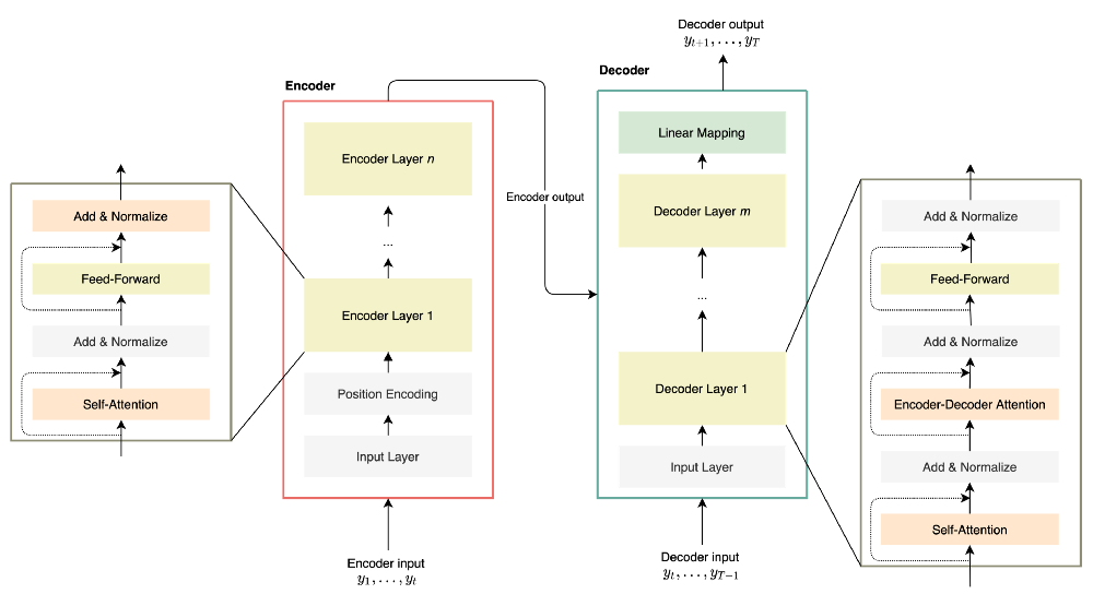
A Transformer-based model is composed of two components.
Encoder. It encapsulates an input layer and a positional encoding layer that maps the input time series data to a vector. The resulting vectors are transferred to self-attention and feed-forward layers with pre- and post-process blocks in between.
Decoder. It is composed of an input layer and decoder layers that are similar to those of the encoder. The decoder also includes an output layer to map the output of the last decoder layer to the target time sequence.
There is one element worth mentioning: in order to make predictions one step at a time using only previous data points, the model uses a one-position offset between the decoder and target output and a look-ahead mask. What does this mean? It implies that all data points that come after the data point currently being predicted are masked, which prevents the model from cheating.
2. The Traditional Machine Learning Approach
What about standard machine learning (ML) algorithms such as random forests, XGBoost, ridge, and lasso?
2.1. How Can ML Models Be Used for Time Series Forecasts?
The first step is to build the dataset from which the model will learn. Usually, the model learns to predict future values based on recent history. Therefore, features mostly consist of lagged values or aggregation such as rolling means, rolling sum, etc.
Figure 5 illustrates the transformation of raw data to a training dataset for one-step prediction. In this example, the model would learn to forecast future values using all the lagged values.

Figure 5— Building the training dataset, illustration by Lina Faik
Note that it is also possible to add more features related to the date in the training dataset. These features include holidays flags, yearly or weekly seasonality components. For more information, here is an interesting article explaining how such features can be computed.
Moreover, as the training set can contain data from multiple time series, it is possible to add features specific to items and thus enable the model to leverage cross-learning benefits. In the case of stock prediction, these features can be information related to the company such as its industry, its earnings, or financial ratios.
2.2. What Feature Engineering Is Required for Multi-Step Forecasting?
However, the prediction for a longer period of time requires more complex feature engineering. Why?
Imagine we want to build a model that is able to make predictions using all the available data, including lag t-1 or features that are computed using lag t-1. In this case, when predicting day+2, these features will be missing since the model has also to predict day+1.
There are two options to deal with this gap:
- Recursive learning. The model can use its last prediction. However, this means that it will learn based on data containing errors from previous predictions and thus quickly accumulate mistakes. Such an approach has great chances to lead to unstable models producing totally inaccurate forecasts.
- Multiple models. The other option would be to build separate models for every time step. In this context, when predicting day+1, we would use a model that is able to make predictions at time t using all lags or related features. When predicting day+2, we would use a model that is able to make predictions at time t using all lags except lag t-1 or all features except those computed from using lag t-1. However, this approach would mean that 30 models need to be trained to make forecasts over the next month! And every model has to be chosen among the available algorithms and its parameters carefully fine-tuned. Therefore, this approach can be very computationally expensive and labor-intensive.
As a good compromise, we consider building one model per week as described in the figure below.
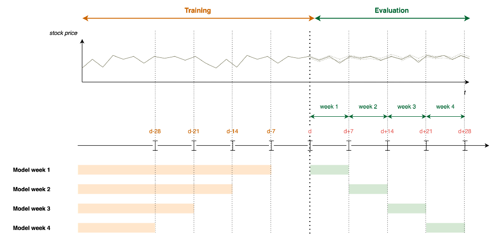
Figure 6 — Learning Framework for an ML approach, illustration by Lina Faik
3. Application to Stock Forecasting
3.1. Scope
The objective of this section is to compare the performance of the models presented above with other approaches in terms of both accuracy and computing time.
It is a continuation of the use case presented in the previous article. Here is a short recap of the main elements that are needed to understand the use case:
Task: Predict the daily stock prices of large companies over the next 30 days.
Dataset: Daily stock price of 100 companies randomly chosen from the S&P index over a period of 10 years. Information about the company is also included (Market Cap, EBITDA, Price/Earnings, Dividend Yield, etc.)
Learning Framework: The dataset is split into two: a training dataset and a validation dataset containing the last 30 days’ prices. The experimentation includes 3 different scenarios:
- Baseline: Only prices are given to the model.
- Date Features: Features related to the date are used by the model to take into account weekly, monthly, and yearly seasonality effects.
- Date Features and Covariants: In addition to price and date features, the model is trained using the covariants described above.
Metrics. RMSE, MAPE and, training time.
3.2. Results
In the rest of this section, you will see my key findings as I explored the results:
- The Transformer performs better in terms of accuracy. Figure 7 compares the results of the different approaches on the test set.
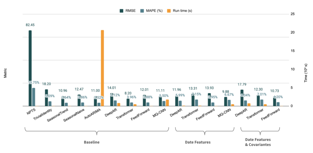
Figure 7 — Results on the test set (expressed as an average over all time series)
Note: Figure 7 presents only averages. In reality, there is a wide disparity of results depending on the company.
2. The ML approach also produces accurate forecasts. Nevertheless, implementing the learning framework is labor intensive as it requires several feature engineering steps and hyper-parameters tuning. Figure 8 contains the results of the different approaches on the validation set (i.e., the last 30 days).
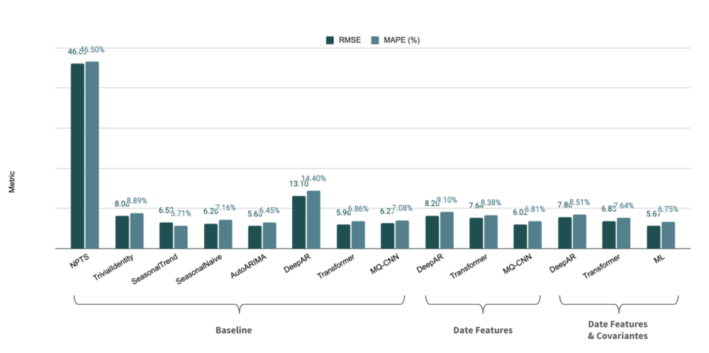
Figure 8 — Results on the validation set (expressed as an average over all time series)
Note: It is worth mentioning that Figure 8 compares the ML approach with other approaches using only one task, i.e. predicting the last 30 days. To properly compare the models and measure the significance of models cores, it is necessary to test them on several points (cf. References).
3. The performance of most models is consistent across forecasting time.
As 30 days represents a long period of time for financial markets, it’s not something to be taken for granted! Table 3 shows the performance of the model depending on the forecasts horizon. For instance, the DeepAR model (baseline) shows a decrease in results for distant time horizons.
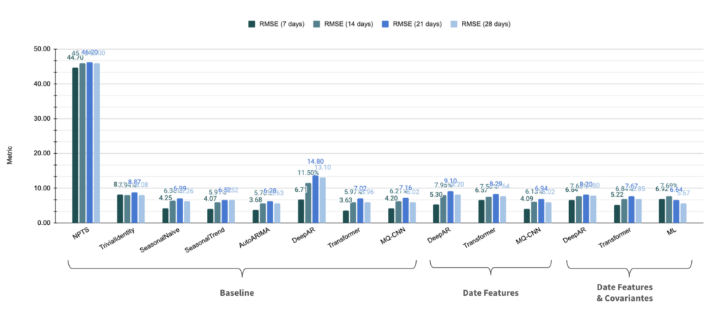
Figure 9 — Results on the validation set depending on the forecast horizon (expressed as an average over all time series)
4. Key Takeaways
Deep Learning vs. Other Approaches: The Final Verdict
Through this two-part series, it appears that forecasting time series using deep learning has many advantages:
- Improved forecast accuracy. By learning global models from related time series, they are able to capture complex patterns and leverage cross-learning between related time series. As a result, the accuracy is higher than state-of-the-art forecasting methods
- Less pre-processing steps and feature engineering. Many research papers have shown that these models work on a wide variety of datasets with little or no hyperparameter tuning. This applies also to datasets of medium size with around one hundred time series.
- No manual intervention during the training phase. Contrary to ML frameworks, deep learning models do not require any specific data pre-processing, feature engineering, or model hand-picking.
- Possibility to include exogenous variables. Contrary to classic statistical methods, deep learning models can include exogenous variables as input variables.
- Reduction of computing time. The architecture of deep learning models enables them to learn and forecast many time series simultaneously.
For all these reasons, deep learning models are much more scalable than other approaches and meet better business constraints in terms of both accuracy and computation time.
The experimentations presented above have been carried out in Dataiku using the plugins time series preparation and time series Forecast in addition to Python code. The trained models are based on the library GluonTS except for AutoArima which is based on the Python library pyramid.
