


Dataiku and UAVIA are working together to push the boundaries of unmanned autonomous vehicles further towards ubiquitous AI and real-time aerial inspections.
UAVIA provides an enterprise-grade software platform that allows industrial operators to integrate autonomous robots, drones, and advanced AI tools into their daily operations. The UAVIA Robotics PlatformTM is a unified environment for drone data management. It can be used for a wide variety of use cases where repeatability, safety, or reactivity are key, such as maintenance or security operations, doubt removal, crisis management, construction monitoring or asset management. Thanks to UAVIA’s DroneOS embedded intelligence, drones can make their own decisions in real time to complete any mission autonomously.
Dataiku, one of the world’s leading AI and machine learning platforms, enables everyone from analysts to data scientists to explore, prototype, build, and deliver their own data and AI products together.
UAVIA’s solutions have been designed to connect with platforms such as Dataiku in order to benefit from the most complex AI models in edge computing and to insure industrial operators are fully sovereign with their data. The collaboration with UAVIA takes Dataiku’s end-to-end platform a step further, enabling any industry to acquire data, organize their datasets, design their models, train, and deploy an optimized variant of their AI for edge computing, allowing drones and robots to detect, inspect, and track a series of objects of interest through time.
Here, we will detail how we used Dataiku to design and train a single shot detector (SSD) model that allows unmanned aerial vehicles powered by UAVIA’s embedded intelligence to automatically detect and track objects of interest in the most hardware-optimized way. In addition, we provide a technical description of the SSD model and present the method we’ve used to simplify the optimization of neural network models for inference within UAVIA DroneOS, using the drone’s specific System On Chip (SOC).
A Fast and Accurate Object Detection Model: SSD Architecture Overview
For a quick review of the basic methods of object detection (Exhaustive Search, R-CNN, Fast R-CNN, and Faster R-CNN), please check out this article. We discuss Fast R-CNN and its nearly state-of-the-art accuracy. However, accuracy isn’t the only metric to take into account, especially when working with real-time prediction. As a matter of fact, depending on the use case, being able to have a fast prediction might be more important than being 2% or 5% higher in accuracy, if not mandatory.
Even though we saw some improvements for time inference with Faster R-CNN, it is usually not enough to score a live video. Two fast object detection models came to the rescue: YOLO (You Only Look Once) and SSD.
YOLO or SSD are preferable over Faster R-CNN for the application of this partnership, given their compromise between inference speed (FPS) and accuracy (mAP). It is known that the performance between the two models are similar in terms of speed and mAP. We decided on SSD due to its easy deployment on drone architecture.
The different algorithms seen in the previous article are called two-shot detector models, meaning they have two stages:
- Region Proposal Stage: Extract a few regions of the image where an object is probably present.
- Classification: Classify the object inside each proposed region and rectify the final prediction location.
SSD, on the contrary, has only one stage. There is no region proposal stage, that is why it’s called Single-Shot Detector. Indeed, it predicts the boundary boxes and the classes at once, directly from the feature maps. To be more precise, SSD makes use of a series of convolutions to predict objects directly from the feature maps of its micro-architecture (a pretrained model that is used as a base model).
Let's Look at an Example
Let’s take an example with an input image of dimension 300x300x3 (width x height x number of channels, which are the three primary colors in our case).
SSD can be implemented using different “backbones” or micro-architectures that serve as a feature extractor. In practice, backbones that make use of separable convolutions, such as MobileNetV2, score better than models using full convolutions in real-time performance. However, for the sake of this explanation, let the simpler VGG-16 be the pretrained model from which the SSD network will extract the features maps. Figure 1 shows the VGG-16 architecture:
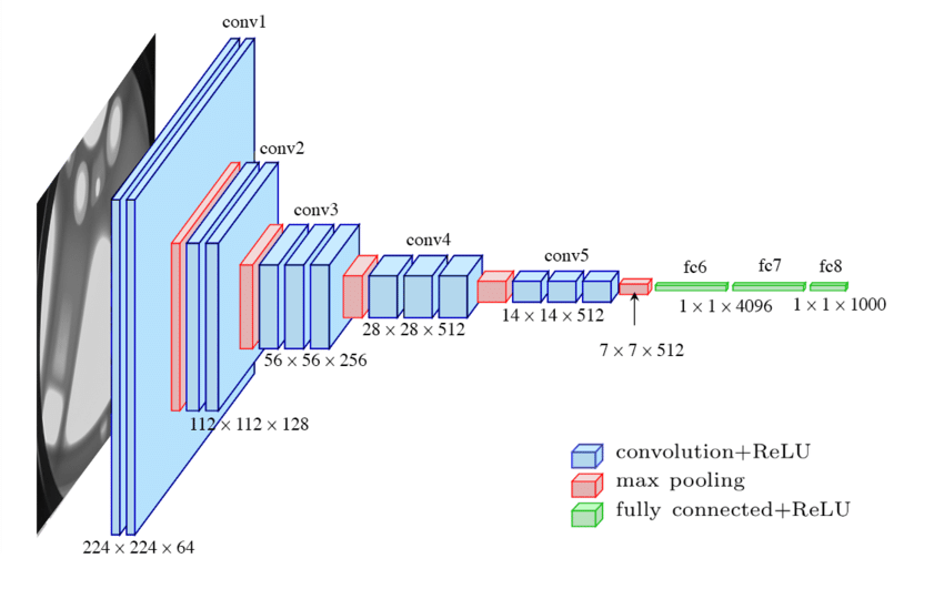
Figure 1: VGG-16 architecture; source
Since we need an image-like output to localize any possible object over an actual image, the last fully connected layers of the VGG-16 become unnecessary and are, therefore, removed from the model. SSD may then use the remaining image-like outputs on different levels of VGG-16 to perform the object detection task.
How Does It Work in Practice?
Let’s take the feature map of the Conv4_3 layer. Following the specifications of VGG-16 paper for the intermediate convolutions and max poolings, the output shape of the Conv4_3 layer will be 38x38x512. The intermediate pooling operations radically change the input spatial dimensions (pixels) from 300x300 to 38x38, while the convolutions increase its depth dimension (channels) from 3 to 512 by applying multiple filters.
For each one those 38x38 pixels, SSD will try to detect objects by testing B default anchors with different aspect ratios. These “anchors” are default boxes classified depending on whether they contain an object of interest or not, see Figure 2.
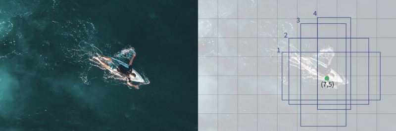
Figure 2: The image represents a set of four default anchors over the position (7,5) on where the SSD will try to identify known objects.
As part of the inference process, SSD may also detect slight modifications to these default boxes that better approximate the real object’s shape, yielding a more accurate result. The object detection task may be seen as two operations that are happening simultaneously: (i) classification and (ii) box regression.
The classification operation (i) aims to recognize the object inside each default anchor as a member of one of our C known objects or as background. Therefore, it classifies each anchor as being part of C + 1 possible categories. The regression task (ii), on the other hand, is intended to better approximate the initial default anchor to the object’s current state by adjusting four output parameters.
Hence, there are C + 1 + 4 anchor parameters to be optimized for each default box. Considering again the output of the Conv4_3 layer (38x38x512) and the B default anchors, SSD will output 38x38xBx(C+1+4) parameters that will determine if (i) there is an object present on the image, (ii) where it is located, and (iii) to which class it belongs.
Consider four different aspect ratios for each pixel on the output and 80 object categories (including the background), we will have:
38 * 38 * 4 * 84 = 485,184 parameters
But how do we actually get those predictions? SSD determines its predictions by a regular convolution centered at each default anchor. Let K be the convolution window size, then SSD will determine its prediction by convolving the output of its backbone with a KxKx512xBx(C+1+4) kernel.
How to Make Use of Different Layers With Multi-Scale Features
Note that, until this point, SSD is considering a fixed size kernel with a fixed size feature map: the Conv4_3 layer. Besides the robustness of the method described so far, it would only be able to detect objects with a compatible size to the representation level acquired at the output of Conv4_3 layer. Objects that, at this level, are bigger than the KxK convolution window applied by the SSD will not be detected at the given layer.
Thinking in this direction, SSD adds a few layers to the pretrained model with the goal of generating different spatial resolution feature maps over which it will perform its prediction. Known as multi-scale features, this will allow the detector to identify objects with different sizes — from big ones that do not fit the convolution window in the early levels of the backbone to small objects that didn’t succeed to reach the end of the model.
Figure 3 shows that the procedure applied to the Conv4_3 is then similarly applied to the added convolutional layers: Conv7, Conv8_2, Conv9_2, Conv10_2, and Conv11_2.
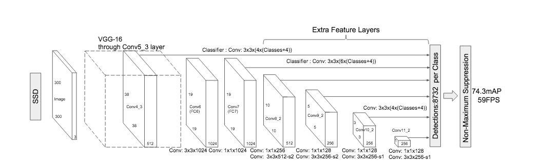
Figure 3: The image presents the SSD performing different detections on different levels of its backbone. Note that the number of default anchors may change from one level to another.
Considering the backbone presented at Figure 4, 80 categories (including the background) and number of default anchors per cell intercalating between six and four for each spatial dimension change, we would have:
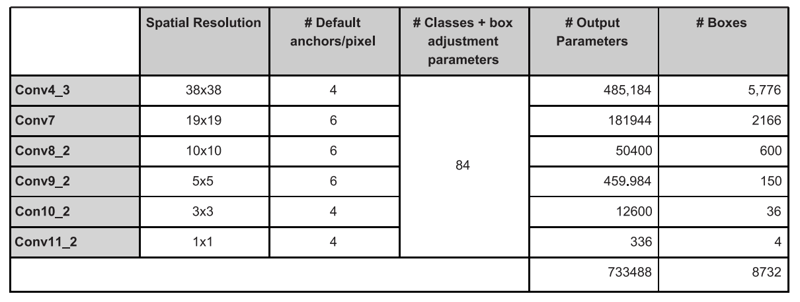
Figure 4: If you are scared about the number, read the comment.
The accuracy is indeed improved when working with multi-scale features. The table below, extracted from the original article, shows how the use of different multi-scale features configuration affects the mAP metric:
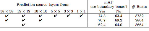
Source: SSD paper
What Is the SSD Model Trying to Optimize?
Neural networks are known for being an AI approach strongly based on multi-objective optimization techniques. As such, they acquire knowledge by trying to minimize the error between their initial predictions and the reality observed in the real world.
This discrepancy has to be encoded by a single function representing numerically the learning direction that the neural network should walk in order to acquire knowledge. The function that encodes this information is called loss function.
An object detection model needs to learn two things: (i) which object we are facing and (ii) where it is located. In this sense, SSD loss function composes the information into a number by a weighted sum of two different losses:
The localization loss: Measures the precision between the ground truth and the predicted boxes. This function considers only the “positive matches,” meaning that it looks at a predicted box only when it has an IoU (Intersection Over Union) greater than 50% with their associated ground truth. Mathematically speaking, this function is usually computed by a Smooth-L1 loss. The closer the predicted box containing the predicted object is to the real box containing the real object, the smaller is this loss.
The confidence loss: Measures the precision of the classification task. This loss encodes how close the prediction class distribution was from categorizing the given object in the right class. Mathematically speaking, usually a softmax function is applied over the output of the network, in order to highlight its predictions, followed by a cross entropy against a binomial distribution representing the ground truth classification. The closer the predicted classification is to the real object’s class, the smaller is this loss.
SSD Improvements and Drawbacks
Last, but not least, SSD also employs several well-known techniques to improve its performance:
- Hard Negative Mining: Several default boxes are going to be generated with different aspect ratios, as presented earlier. Many of these boxes will not contain any object. Others will maybe wrongly categorize them or not correctly predict their bounding shape. Considering the number of boxes tested per image, very likely the majority of our predictions will be composed by negative detection (boxes classified as not containing any object). If the SSD incorporates all these boxes in its learning process, its learning will be biased towards detecting that no object is present at all most of the time. Hard negative mining allows us to correct this by keeping only part of negative matches with the highest losses. SSD sets a proportion of 3:1 to determine how many negative matches are allowed to be back-propagated. That is, three negative matches for each positive match.
- Data Augmentation: Training datasets are usually limited in one way or another. It is extremely difficult to represent every possible real-world case in a limited number of samples. For this reason, several papers add a data augmentation step where they try to vary their input training images by flipping, cropping, or modifying their color histograms. SSD’s paper shows that this procedure increases its mAP by almost 9% when using the VOC2007 dataset.
- Non-Maximum Suppression (NMS): Finally SSD applies NMS function, just like Faster R-CNN, where the idea is to identify and delete overlapping boxes predictions that probably belong to the same object.
SSD works well, really well actually! However, there are two drawbacks we can make:
- The accuracy performance with small-scale objects can be altered. The reason is that the small objects are detected in high resolution layers, where there is less information.
- SSD does its best to detect objects over images as fast as it can, even though it means sacrificing part of its accuracy. However, this accuracy loss may mean that an object will be missed from time to time. It might not be an important issue in a fixed frame analysis. But when performing detection over a sequence of temporally dependent frames, this lack of detection arises intermittent detections and interferes with the overall video analysis.
Object Tracking
To illustrate some of these difficulties, consider a drone flying at a height of about 40 meters. For this drone, everything on the ground would look pretty small. Combine that with input images of size 300x300 pixels and your objects might be only ten pixels long, as can be seen in the following “camera versus resized” comparison:
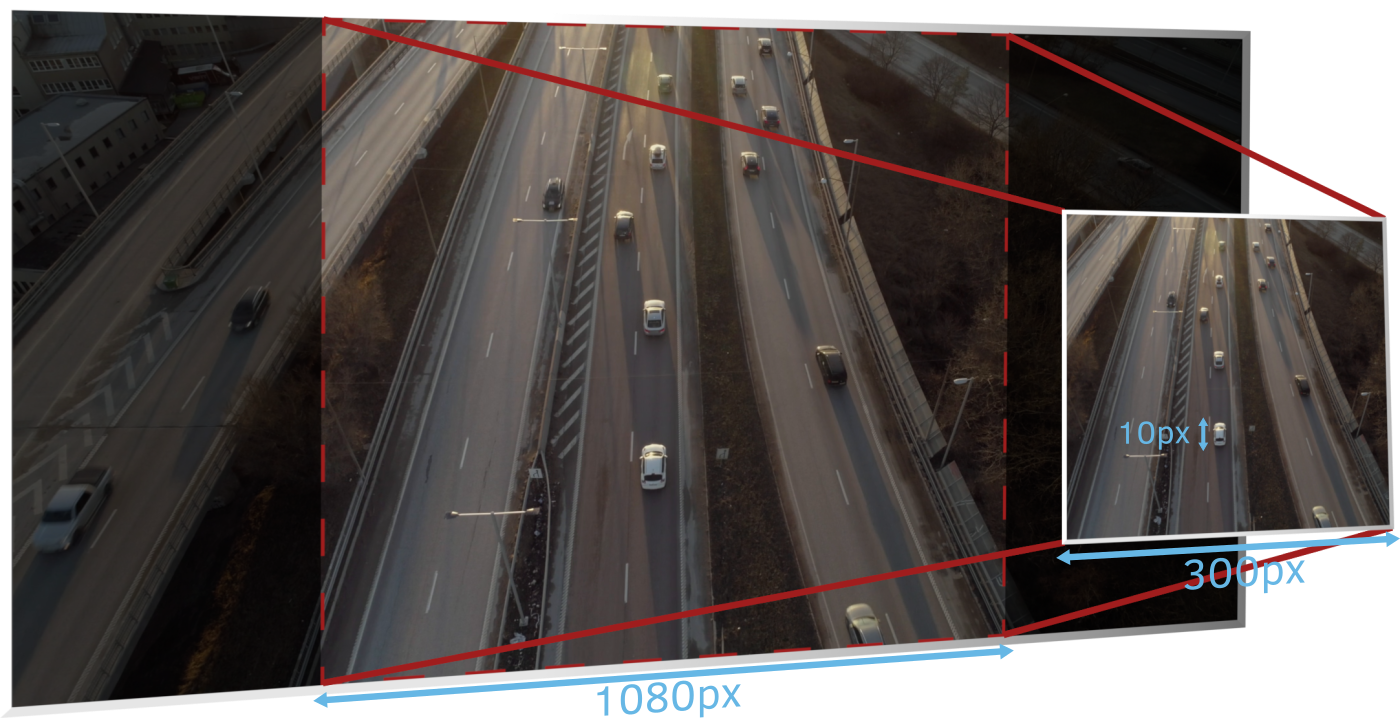
Figure 5: Comparison between the captured image (with an already small object representation) and the downsampled version used as input to the SSD model.
This makes the task very challenging. Objects easily go undetected (false negatives), while the risk of wrong detections increases (false positives). Regardless of the model type, one way to mitigate this issue is to post-process the detection results through a tracker. The role of the tracker is to assign an ID to detected objects, and to consistently assign that same ID to detections of the same object from one frame to the next. We will explain how this can help improve the detection results.
Not only that, but it also enables autonomous drones to better exploit detections. For example, since the drone can recognize an object by its ID, it can follow it around on its own. This ID assignment problem, a.k.a. Data Association Problem, can be formulated as a “minimum cost flow” through the following graph, from source to sink:
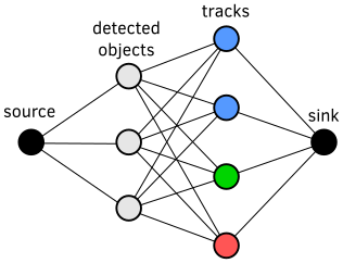
Figure 6: Flow graph representing the ID assignment problem (also known as a data association problem). The flow starts from the source towards the sink (black nodes). Known objects (gray nodes) are connected to new detections (blue and green nodes) and a clutter possibility (red node). Each known object may use at most one edge to flow from source to sink.
The detected objects on the current frame are on the left side of the graph. The goal is to assign them optimally to nodes on the right side of the graph which consist of:
- Blue nodes: A detection from the previous frame. If a new detected object is assigned to a blue node, it inherits the ID of the older object.
- Green node: A new object not previously detected. In this case, a new ID is generated for the object.
- Red node: A false positive, or clutter. The detected object is discarded and its bounding box will not be displayed.
The costs of each assignment are calculated taking into account detection data such as scores, labels, overlap between bounding boxes, and predicted positions of previously tracked objects. A small object that is detected with a low score, and would usually be considered clutter, can now still be matched to a previously detected object if they strongly overlap.
The tracker enables the use of imperfect but fast real-time object detection models to obtain great results in situations where the models themselves might struggle. False positives are largely eliminated, and if a tracked object is suddenly not detected for just one frame, it can still be displayed from its predicted position evaluated with methods such as Kalman filters, making the bounding box appear more consistently.
Watch this in action in this comparison video:
Let’s Build Our SSD Model
In order to put theory into practice, we use Dataiku to train our object detection model using the TensorFlow Object Detection API. It is an open source framework built on top of TensorFlow that makes it easy to construct, train and deploy object detection models. To install it, please refer to this link.
Pretrained Model
As we have seen previously in the SSD explanation, the user has to choose a pretrained model. For the sake of this presentation, we used MobileNetV2 which has been trained on the COCO dataset. For our current task of dealing with ML on drone, MobileNetV2 seems to be a good fit since it is fast and does not lose too much accuracy. Indeed the MobileNet neural network family has been released by Google and is first meant to be used on machines with limited computing power.
Model Settings
You can follow the next steps using the code from this tutorial. You have to create or edit a few files before your model is ready to be trained:
- Label map (JSON file mapping your ID to the name of your class)
- Training configuration file. You can start from an existing one and modify it as you wish. You will have to fill the number of classes you are using and the paths to your pretrained model, labeled dataset, and images.
Packaging the Model for Deployment
Once the model is trained and ready to be deployed, it is time to send it to UAVIA DroneOS. We package all the model files together and upload them to a shared storage server. Among the different possible ways to store and transfer data, we use a Docker registry.
Make the Model Readable by the Drone
With the object detection model trained and provisioned to UAVIA DroneOS though UAVIA Robotics PlatformTM, we are ready to fly, right? Well... not just yet. In order to squeeze as much performance as possible out of the embedded SOC, the models first must be converted and optimized.
TensorFlow and PyTorch are great frameworks for training neural networks. But when it comes to inference, they are not the best tools for the job, particularly if you want to use hardware capabilities at their maximum. For instance, specialized libraries such as Nvidia’s TensorRT allow us to optimize neural networks for inference on GPU. In the embedded world, Nvidia has a family of boards known as Jetson with powerful ARM processors and a fully operational GPU on-board.
From an AI perspective, drones are flying GPUs. As you may know, the world of machine learning is in constant evolution. New neural network architectures, new layers, and new needs are emerging everyday. Unfortunately, TensorRT is lagging a little bit behind TensorFlow and PyTorch. However, it is still possible to convert your cutting edge TensorFlow object detection model to TensorRT if you are willing to put some work into that. In fact, this is one of the services UAVIA provides to its clients.
More than that, the Jetson family is not the only hardware for drones out there. UAVIA has an internal framework that allows it to easily deploy any trained model from Dataiku to some of the main inference frameworks such as TensorRT, OpenVINO, OpenCV and TensorFlow Lite.
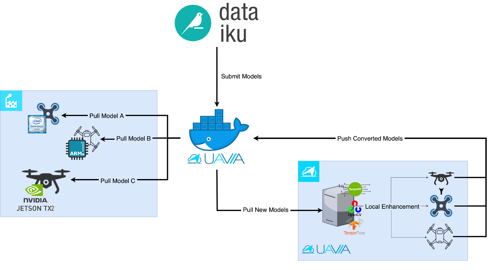
Figure 7: Flow diagram presenting UAVIA’s model optimization pipeline to deploy Dataiku’s trained models on drones.
Next, we will talk about the conversion to TensorRT. For other configurations, such as a drone with an Intel Movidius inference accelerator and the Intel OpenVINO library, the conversion process is broadly similar, although the details may vary.
The overall process is illustrated in the following figure:
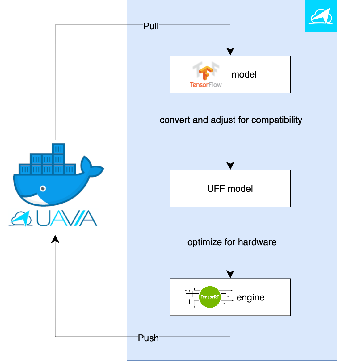
Figure 8: Flow diagram showing UAVIA’s model optimization pipeline for TensorRT.
For the most cutting edge models, TensorRT cannot directly perform inference from TensorFlow implementation. This is the case for the model trained above on the Dataiku platform. It first needs to be converted into a Universal File Format (UFF). Unfortunately, TensorRT does not provide implementations for some neural network layers. When this is the case, we implement a TensorRT plugin ourselves in order to provide the missing functionality. For example, plugins are used for flatten-concat, NMS, and grid anchor generation. Such compatibility adjustments have to be baked in, at the stage of the conversion, to UFF.
The resulting UFF model file can be loaded in TensorRT and used for inference. However, the model optimization process does not end here. TensorRT is indeed able to parse a UFF model, but it also performs hardware specific optimizations. For example, it fuses multiple layers into a single Cuda kernel which results in increased memory bandwidth, and selects the kernels that perform best on the target hardware. The result of this optimization is called a TensorRT engine model. This engine is the final form of the model that can be used on drones for the best performance. It is packaged and published to the model library on the server, ready to be deployed.
All these steps only need to be performed once. Once we have the TensorRT engine available, we can deploy it on as many drones as we like, as long as they match the hardware that it has been optimized for. The process described here is automated in production, such that once a model is trained on Dataiku, it can automatically be converted and optimized for UAVIA DroneOS running on the target SOC of the client's drones.
Real-Time Inference by UAVIA’s DroneOS
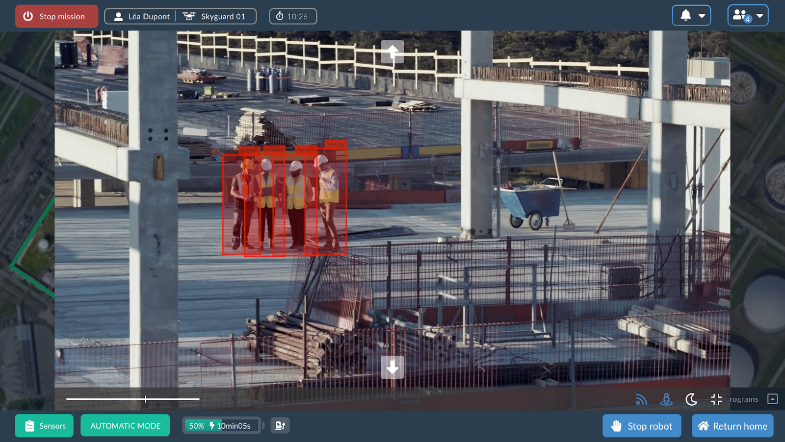
Once the TensorRT engine model is on a drone and ready to be used, performing inference is only one click away. In any UAVIA application, whether on a computer, tablet, or phone, the video feed from the drone’s camera is displayed in real time and features a button to toggle object detection on and off.
Figure 9: Real-time object detection (workers on a construction site) streamed directly from the drone to UAVIA’s web application. All the image processing, drone navigation, and object detection inference are processed in the autonomous drone.
The computer vision pipeline features are image stabilization, object detection (e.g., using the model that was optimized above), and tracking. For the end user, the experience is seamless, allowing them to focus on the essentials. The drone can be controlled by simply clicking on the target location on the map.
Beyond what was presented here, object detection enables other interesting use cases. For example, a drone mission can be completely pre-programmed, executed automatically at scheduled times, and report any detections that it made during its routine inspection flight.
Conclusion
This use case is a good example of a real-life ML pipeline for edge computing. It also shows us the advantages of using Dataiku and UAVIA to create such a pipeline.
With Dataiku, users can:
- Easily label images if needed and make the data ready to use
- Train deep learning models and retrain them automatically when more images become available
- Ensure the data quality and the model performance before sending it to the drone
With UAVIA, users can:
- Automatically convert and optimize a model for inference on a drone's embedded hardware
- Deploy models to a fleet of drones, each with different hardware
- Run real-time object detection inference and tracking during flights using UAVIA web application telemetry