


In addition to the most popular unsupervised learning technique — clustering — there is dimensionality reduction, which we’ll cover in the latest article of our “In Plain English” blog series, designed to make data, data science, machine learning (ML), and AI topics accessible to non-technical experts.


As a reminder, unsupervised learning refers to inferring underlying patterns from an unlabeled dataset without any reference to labeled outcomes or predictions. Clustering refers to the process of automatically grouping together data points with similar characteristics and assigning them to “clusters.” Dimensionality reduction, on the other hand, refers to a set of techniques that reduces the dimensionality — or, number of features — in your dataset. Let’s take a closer look.
Why Do We Need to Reduce Dimensionality?
It may be tempting to just throw as many features as possible into your model (more data is better, right?), but it’s very important to understand the shortcomings that go along with including too many features in your model. These shortcomings are collectively known as the curse of dimensionality.
The key downfalls associated with having very high-dimensional datasets include:
- More data necessary – In order to ensure that every combination of features is well represented in our dataset, we’d need more records of data.
- Overfitting – The more features a model is trained on, the more complex our model becomes and the more we risk poor assumptions and potentially fitting to outliers.
- Long training times – Larger input datasets mean more computational complexity during model training and longer training times.
- Storage consumption – Larger datasets require more storage space.
We can try to get more data or more powerful machines with larger storage capacity, but this is not always possible or sufficient to solve the problem. If we took a cube to represent a three-dimensional dataset with 1,000 data points and projected it onto a two-dimensional plane, we would only see one face of the cube. This improves visualization, as it’s easier to see a graph in a two-dimensional space than in a three-dimensional one and, with ML algorithms, it takes less resources to learn in two-dimensional spaces than in a higher space.
Dimensionality Reduction in Action: Practical Examples
Let’s imagine we’re going to build a model to predict how much money an individual customer will spend at our store — Willy Wonka’s Candy — this week. We have a large dataset with customer demographics as well as information on how much they spent on all of the candies at our store last week.
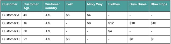 Figure 1
The above is just a very small snapshot of a handful of rows and columns, but let’s imagine that this dataset actually had hundreds or thousands of columns. Some of these columns may be completely unhelpful in predicting customer spend, while others may have quite a lot of overlap and won’t need to be considered individually. For example, maybe we can combine Dum Dums and Blow Pops to look at all lollipops together. Dimensionality reduction can help in both of these scenarios.
There are two key methods of dimensionality reduction:
- Feature selection: Here, we select a subset of features from the original feature set.
- Feature extraction: With this technique, we generate a new feature set by extracting and combining information from the original feature set.
Feature Selection
Let’s imagine our dataset also has a column on customers’ favorite movies, and we realize that this is not incredibly useful in helping us predict how much they’ll spend at our store. With feature selection, we’d just exclude this entire feature. This particular example might be obvious, but that isn’t always the case. We can perform feature selection programmatically via three key methods: wrapper, filter, and embedded methods.
Wrapper Methods
Wrapper methods iterate through different combinations of features and perform a model retrain on each. The feature combination which resulted in the best model performance metric (accuracy, AUC, RMSE, etc.) is selected.
Two key wrapper methods include:
- Forward selection - Begin with zero features in your model and iteratively add the next most predictive feature until no additional performance is reached with the addition of another feature.
- Backward selection - Begin with all features in your model and iteratively remove the least significant feature until performance starts to drop.
These methods are typically not preferred as they take a long time to compute and tend to overfit.
Filter Methods
Filter methods apply a threshold on a statistical measure to determine whether a feature will be useful. Two key methods include:
- Variance thresholds - Remove any features that don’t vary widely. For example, in our Willy Wonka dataset, we can see that all of our customers live in the U.S., so that feature would have a variance of 0, and we’d likely want to remove it.
- Correlation thresholds - Remove highly correlated features, as the data is redundant. For example, let’s imagine that we also had a year of birth column in the above dataset. This would be highly correlated with our age column and would not be helpful in generating any stronger predictions.
These methods are very straightforward and intuitive. However, they require manual setting of a threshold which can be dangerous, as too low of a threshold may mean the removal of important information. Additionally, these two methods are often not sufficient if we want to seriously reduce the dimensionality of our dataset.
Embedded Methods
Certain ML algorithms are able to embed feature selection into the model training process. Key embedded methods include:
- Regularized linear regression - These methods add a penalty that corresponds to the value of the coefficients. This way, coefficients with lower predictive power are weighted less heavily, and the overall variance of the dataset is reduced. There are two key types of regularized linear regression:
- Lasso regression - In lasso regression, also referred to as L1 regularization, the penalty is equivalent to the absolute value of the coefficient. This means that coefficients of unimportant features can be reduced to zero, which effectively eliminates them from the model.
- Ridge regression - In ridge regression, also referred to as L2 regularization, the penalty is equivalent to the square of the coefficient value. Because coefficient values are squared, coefficients cannot be entirely eliminated from the model, but can be weighted less heavily.
- Regularized trees - When building tree-based models, we can use metrics like entropy (discussed in our tree-based models post) to measure feature importance and can then elect to only keep the top N most important features.
Embedded feature selection combines key features of wrapper and filter methods and is often a great place to start, as long as you’re using a compatible algorithm.
Feature Extraction
Feature extraction allows us to keep parts of features, so that we just keep the most helpful bits of each feature. This way, we don’t lose too much information by removing entire features. Principal Component Analysis (PCA) is far and away the most common method of performing feature extraction and is the method we’ll explore in this post.
PCA
The purpose of PCA is to reduce the number of features included while still capturing the key information, or the spread of the data, as measured by the variance.
We’ll generate this new, smaller feature set by linearly combining the features within the original feature set. The new features are called principal components. The first principal component is the line which captures the majority of the variance within the dataset, and the second principal component captures the second most variance, and so on. Each of these principal components is orthogonal to the next — this means that they are uncorrelated. In two dimensions, this would be equivalent to perpendicular angles. See Figure 2 below.
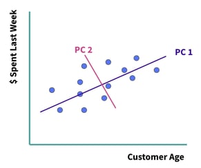 Figure 2
There are two key methods of computing the principal components — eigendecomposition and singular value decomposition (SVD). The details of these methods are beyond the scope of this blog post, but the key is that either way, we’ll find principal components in decreasing order of variance. Additionally, prior to computing the variance — and regardless of the method we use — we’ll want to ensure that the dataset is normalized to account for potentially varying units of measurement.
If you have a dataset of m features, you’ll initially create m principal components. Then, you may want to only keep the principal components which add up to, say 90% explained variance, and you’ve then reduced the dimensionality of your dataset by removing the least significant principal components. In Figure 3 below, you’ll notice that there’s a fairly steep drop off in explained variance after principal component 4, so it may make sense to set a threshold right there, as marked.
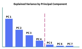 Figure 3
PCA is very fast and works well in practice. However, it does obscure your features, so rather than looking at, say Twix sales, you might be looking at principal component 2, which is some combination of Twix sales along with several other features. If interpretation is important, unfortunately PCA will likely be problematic. However, if it’s not important, PCA is an excellent way to programmatically reduce the dimensionality of your dataset.
Recap
Including too many features in your dataset can be problematic, a problem referred to as the curse of dimensionality. Essentially, you’ll need more data, risk overfitting, and potentially run into computation or storage problems.
Dimensionality reduction can help you avoid these problems. The key dimensionality reduction techniques can be broken down into two key categories: feature selection (selecting specific features to include) and feature extraction (extracting a new feature set from the input features). The method that will work best depends on your particular dataset and business objectives, but dimensionality reduction can be an excellent data preparation method, especially when working with massive datasets!