


ML outcome optimization is the process of finding optimal feature values that give the model prediction minimum (or maximum) over a defined space. For black-box ML models, we cannot assume any of the usual smoothness properties for optimization, such as convexity or even differentiability. Therefore, powerful standard optimization techniques, like gradient descent, are not applicable, and it is common to use meta-heuristics such as evolutionary algorithms.
Evolutionary optimization is inspired by natural selection to find the best solution to a problem. It relies on the building block hypothesis or, as Wikipedia states it, they perform adaptation by identifying and recombining “building blocks,” i.e., low order, low defining-length schemata with above average fitness. However, as there is no guarantee to reach the global optimum, evolutionary methods usually iterate until a computation budget is exhausted or there is no more improvement after a given number of iterations (think early stopping).
A famous example of outcome optimization available on OpenML is the selection of the most optimal quantities of ingredients to create the sturdiest concrete. The dataset is composed of measures of the resistance of various mixing of concrete after different drying delays. We wish to maximize this resistance over time.
The Need for Diversity
Most outcome optimization methods available on the open source market do not care about diversity and simply run until their stopping condition is met, then return the best sample found so far. We believe, however, that diversity can lead to great improvements for four reasons:
- Exploration / exploitation trade-off. Sometimes several close-to-optimal solutions can have drastically different feature values. For example, the top mixes already present in the dataset are very close with very different compositions in the concrete mixing dataset.
- It is not expensive. Evolutionary techniques must explore the sample space enough not to miss a potential minimum. It means that several local minima will be explored during the optimization process. Enforcing diversity can be as cheap as remembering those local minima.
- The model is not perfect. Outcome optimization seeks for the global minimum of a model prediction. But the model prediction is not perfect and, in the end, only a human expert can determine the value of a proposition. Returning a diverse set of samples increases the chance to find the best option.
- Results may not be plausible. Outcome optimization is often applied to physical processes, such as concrete mixing, that obey physical laws that the system may not entirely know. We increase our chances of returning a realistic one by returning several different samples.
Warning: In this post, to avoid causality and plausibility concerns, we assume that all features are causally independent mechanisms.
Building Units of a Genetic Algorithm
But first, let’s review how genetic algorithms work. Genetic algorithms consider a set of candidate samples as a population of individuals and make them evolve through three life-like processes:
- Mutation of the existing population. We apply small mutations to existing individuals to explore their immediate surroundings.
- Recombination of individuals. We mix the genetic material of two individuals to create children, hoping that some of them will have a better score.
- Extinction of weak individuals and birth of new populations. At each iteration, the weakest individuals of the population are removed and replaced by newly drawn ones. Contrary to the mechanisms described above that generate samples next to existing ones, we renew the genetic material by simulating the arrival of a new population based on pure exploration.
Genetic algorithms do not always implement all of these functions. For example, scipy’s differential evolution algorithm relies only on recombinations and does not propose pure mutation (contrary to what its parameters suggest, the mutation parameter controls the scale of recombination). Because recombinations rely on existing solutions only, it may hurt plausibility or lack exploration power. For this reason, we have decided to stick to mutation and exploration operators for our algorithm.
Initialization of Random Individuals
Random individuals are sampled uniformly between the minimum and maximum of the continuous variables and from all possible categories for categorical data.
Mutation of Individuals Through Local Exploration
Mutations are slight changes applied to one sample, in the hope that newly generated ones will have better fitness score. Just as in scipy, we propose to use an exploration weight to control the perturbation of each feature following the procedure:
- Categorical features. The weight corresponds to the probability of changing the feature. If the feature changes, a category is drawn from the category distribution of the data.
- Numerical features. We consider a normal distribution centered on the reference value for the feature and of standard deviation equal to the standard deviation of the data scaled by the weight.
Life and Death of a Lineage
As mentioned before, integrating diversity in outcome optimization is the occasion to explore local optima. It means that we must explore several local minima in parallel. To this end, we create the concept of lineage inside our algorithm:
- A newly created sample through exploration starts a new lineage.
- Each time this sample mutates, the resulting mutations belong to the same lineage.
- If a lineage fails to improve over a certain number of iterations, it goes extinct and its best representative is kept in a cache.
At the end of the procedure, we perform a K-Means clustering on the cache and return the best representative of each cluster, promoting diversity.
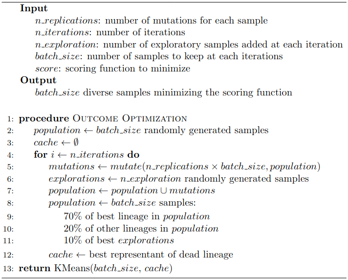
A Pseudo-Code Is Worth a Thousand Words
Outcome Optimization in Action
We visualize our algorithm’s behavior on a simple one-dimensional function. Our goal is to find the minimum of the blue function presented below. Moving points are the individuals at a given iteration (the movements are not that slow, we interpolated them for the visualization). Once a lineage expires and is sent to cache, we display its best representative with a gray cross.
For each lineage, we indicate the score of its best current representative in the middle of the figure. The line turns gray when the lineage has been sent to the cache and the score cannot improve anymore.
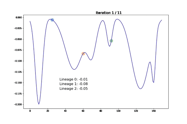
Note that, for this experiment, we voluntarily chose hyperparameters so that samples have a smooth trajectory. Here, we observe that samples tend to “climb down” their hill until their local minimum. Once this minimum is reached and the lineage cannot improve, we send it to cache and plot it in gray. We then add a new lineage starting in a random location. In the last iteration, we see that most local minima have been explored. We can therefore return a pertinent set of diverse samples.
Perfect Concrete Mixing: The Need for Plausibility
Let’s apply our method to find the best concrete mixing.
Concrete is the most important material in civil engineering. The concrete compressive strength is a highly nonlinear function of age and ingredients. These ingredients include cement, blast furnace slag, fly ash, water, superplasticizer, coarse aggregate, and fine aggregate.
How to Measure Concrete Resistance
Concrete resistance is measured in compressive strength expressed in MegaPascals. The strength of concrete tends to increase in the first days due to the drying process and then goes down when the concrete starts aging. In this example, we are interested in examining the resistance during the drying process. Because the resistance in the early days can be different than the final resistance of the concrete, we are looking to maximize the area under the resistance curve:
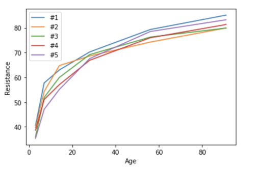
In this plot of the resistance of the top five concrete mixes, we can see that the orange one is the most resistant concrete on day 15, but the least resistant one on day 100.
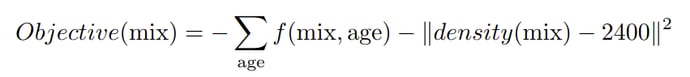
Given our model f, we wish to minimize the following objective:

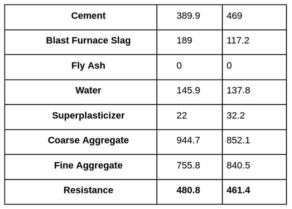
For this exercise, we use an MLP with three hidden layers of size 32 but the method is agnostic with respect to the model. The result is astonishing: Our generated samples are way better according to our model!
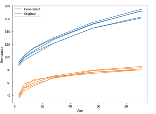
However, they are so good that it raises suspicions… The units of ingredients in the mixing are expressed in kg/m³, and there is a physical limit to the weight we can put in a cubic meter of concrete. According to Wikipedia, the density of concrete varies, but is around 2,400 kilograms per cubic meter.
And this is verified in the original data, while our generated data is way off!
Top five original densities: 2447.3 | 2448.8 | 2405.9 | 2463. | 2460.
Top five generated mixes densities: 3220.3 | 3228.0 | 3201.8 | 3036.5 | 3047.1
For now, our toolbox does not allow for the generation of realistic samples. Plus, given how genetic algorithms work, it may be beneficial to keep some unrealistic samples for further mutation to explore more options!
We therefore push our algorithm to keep more realistic mixes by penalizing samples going too far from the average density of the concrete.
The density of newly generated mixes is much more realistic and, unfortunately, the concrete obtained is much less performant, but we still found a way of improvement!
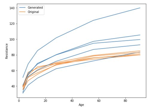
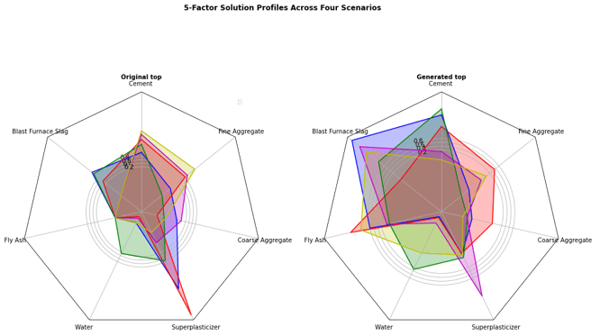
Looking at the generated samples, we obtain very diverse samples with mixes that include entirely different ratios of ingredients!
Takeaway
In this task of finding the optimal quantities of ingredients to create the sturdiest concrete, we confirmed that adding plausibility was necessary to get valid results. We also found that adding diversity was cheap and a good way to offer several options to the user whom may hold information that the model does not. We believe that further research regarding diversity could lead to even better outcome optimization methods.
This feature, including its diversity enforcement, can be found in Dataiku 11, which will be released soon!