


A core assumption necessary for causal inference is the positivity assumption (have a look at our other post for a discussion on the main assumptions necessary for causal inference). This is the assumption that, for every subgroup of your data, all kinds of treatment are present in that subgroup. For binary treatment, that means:

This is also called the “common support assumption” because the conditional distributions P(T = 1 | x) > 0 and P(T = 0 | x) must share a common support.
If this assumption isn’t true, when we try to estimate causal effects by estimating P(T = t | x) or E[Y | t, x], we will be extrapolating in regions where P(x) > 0 and P(t | x) = 0. Here’s an illustration of that from a causalcourse.com lecture on positivity:
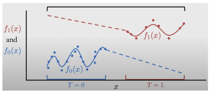
The dots are data points and the dotted lines correspond to where the model of P(t | w) will be extrapolating.
To intuitively understand this, let T = 1 correspond to treated and let T = 0 correspond to control; If we have a subgroup X = x where every unit is treated, we don’t have any data to tell us what might have happened if that subgroup was not treated. See Neal (2020, Section 2.3.4) for more info.
So we need methods that can accurately tell us if the positivity assumption is violated, and, if so, where.
The most common method is estimating P(T = 1 | x) using a classifier such as logistic regression and classifying positivity violations as all values P(T = 1 | x) that are < ε or > 1 - ε, for some ε such as 0.05. This method is studied by Crump et al. (2009) and is called propensity thresholding.
However, there are many other methods for detecting positivity violations. For example, there’s “the IBM method” from Karavani et. al (2019) and “the Vianai method” from Wolf et al. (2021) that we’ll now introduce.
Positivity Violation Detection Methods
Propensity Thresholding:
- Fit a model for P(T = 1 | X) (propensity score).
- Choose a thresholdε and consider all samples with P(T = 1 | X) < ε and P(T = 1 | X) > 1 - ε positivity violations.
Code:
class PropThresholding: def __init__(self, model): super().__init__() self.model = model self.prop_threshold = None def predict_propensity(self, X): """Predict propensity scores for each observation in X.""" return self.model.predict_proba(X)[:, 1] def predict_positivity_violation(self, X, prop_threshold=None): if prop_threshold is None: prop_threshold = self.prop_threshold pred_props = self.predict_propensity(X) pred_violations = (pred_props < prop_threshold) | (pred_props > 1 - prop_threshold) return pred_violations
IBM Method:
- Fit a random forest for P(T = 1 | X).
- For every tree in that forest, check if a sample is in a leaf where all samples in that leaf are all control group or all treatment group; consider a sample a positivity violation if at lease ε trees put that sample in a homogenous leaf.
Code:
import flamlimport numpy as npimport sklearnclass IBMForest: def __init__(self, X, t, rf_type='flaml_default', separate_treat_control=True, max_minutes=2, homogeneity_threshold=0): super().__init__() if rf_type == 'sklearn': self.model = sklearn.ensemble.RandomForestClassifier() elif rf_type == 'flaml_default' or rf_type == 'flaml': self.model = flaml.default.RandomForestClassifier() elif rf_type == 'flaml_tuned': self.model, _ = train_automl_pipeline(X, t, max_minutes=max_minutes, estimator_list=['rf']) else: raise ValueError('rf_type must be flaml or sklearn') self.X = X self.t = t self.separate_treat_control = separate_treat_control self.homogeneity_threshold = homogeneity_threshold self.min_tree_threshold = 0.5 self.model.fit(X, t) def predict_propensity(self, X): """Predict propensity scores for each observation in X.""" return self.model.predict_proba(X)[:, 1] def predict_positivity_violation(self, X, separate_treat_control=None, min_tree_threshold=None,
homogeneity_threshold=None): """
Predict positivity violations for each observation in X. Implements the rule described in Section 3.2.1 of this
paper: https://arxiv.org/abs/1907.08127
:param X: Data to predict positivity violations for
:param separate_treat_control: If False, then the violations are aggregated as described in the paper ("fraction
of times it was counted as a violation"); if True, the positivity violations are computed separately for
treated and control
:param min_tree_threshold: Minimum proportion of trees that must predict a violation for the observation to be
considered a violation
:param homogeneity_threshold: Minimum proportion of observations in a leaf that must be of the same treatment
status for the leaf to be considered homogeneous
:return: A boolean array indicating whether each observation in X violates positivity
""" if separate_treat_control is None: separate_treat_control = self.separate_treat_control if min_tree_threshold is None: min_tree_threshold = self.min_tree_threshold if homogeneity_threshold is None: homogeneity_threshold = self.homogeneity_threshold print('min_tree_threshold', min_tree_threshold) # Get whether each tree in the forest predicts a violation tree_control_violations = [] tree_treatment_violations = [] tree_either_violations = [] for i, tree in enumerate(self.model.estimators_): propensities = tree.predict_proba(X)[:, 1] control_violations = propensities <= homogeneity_threshold treatment_violations = propensities >= 1 - homogeneity_threshold either_violations = control_violations | treatment_violations tree_control_violations.append(control_violations) tree_treatment_violations.append(treatment_violations) tree_either_violations.append(either_violations) # Get the fraction of trees that predict a control violation: P(T = 1 | X) = 0 frac_control_violations = np.array(tree_control_violations).mean(axis=0) # Get the fraction of trees that predict a treatment violation: P(T = 1 | X) = 1 frac_treatment_violations = np.array(tree_treatment_violations).mean(axis=0) # Get the fraction of trees that predict a violation frac_either_violations = np.array(tree_either_violations).mean(axis=0) # For each sample, get the fraction of trees that predict whichever violation is more common: # P(T = 1 | X) = 0 or P(T = 1 | X) = 1 if separate_treat_control: frac_violations = np.array([frac_control_violations, frac_treatment_violations]).max(axis=0) else: frac_violations = frac_either_violations # Threshold the fraction of trees that predict a violation pred_violations = frac_violations >= min_tree_threshold return pred_violations
Vianai Method:
- Fit a model for P(T = 1 | X).
- Bin the P(T = 1 | X) estimates into 100 bins for both the control group and treatment group.
- For each of the 100 bins, use a proportion test to test if that bin in the control group is statistically significantly different from that bin in the treatment group. If so, all samples in that bin are considered as violating positivity.
Code:
import numpy as npfrom statsmodels.stats.proportion import proportions_ztestfrom statsmodels.stats.multitest import multipletestsclass VianaiMethod: def __init__(self, pipeline, X, t, alpha, n_bins=100): super().__init__() self.pipe = pipeline self.n_bins = n_bins # Predict propensity scores prop_scores = self.pipe.predict_proba(X)[:, 1] # Separate propensity scores into treatment and control prop_scores_treat = prop_scores[t == 1] prop_scores_control = prop_scores[t == 0] # Get the totals for each group n_treat = len(prop_scores_treat) n_control = len(prop_scores_control) # Specify the bins and get the histogram counts self.bin_edges = np.linspace(0, 1, self.n_bins + 1) hist_treat, bin_edges_treat = np.histogram(prop_scores_treat, bins=self.bin_edges) hist_control, bin_edges_control = np.histogram(prop_scores_control, bins=self.bin_edges) # Assert that all the bin edges are the same as bin_edges assert np.array_equal(self.bin_edges, bin_edges_treat) and np.array_equal(self.bin_edges, bin_edges_control) # Suspected violations: get bins where there are 0 in treatment and non-zero in control (XOR) or vice versa susp_bin_violations = np.logical_xor(hist_treat == 0, hist_control == 0) # Conduct two-sample proportion hypothesis tests on the bins where there are suspected violations pvals = [] for k_control, k_treat in zip(hist_control[susp_bin_violations], hist_treat[susp_bin_violations]): _, pval = proportions_ztest([k_control, k_treat], [n_control, n_treat], alternative='two-sided') pvals.append(pval) if len(pvals) > 0: # If there are any suspected violations # Use the Benjamini–Hochberg FDR procedure for multiple testing reject, pvals_corrected, _, _ = multipletests(pvals, alpha=alpha, method='fdr_bh') # Get the violating bin indices self.bin_violations_idx = np.arange(self.n_bins)[susp_bin_violations][reject] else: # No suspected violations self.bin_violations_idx = [] def predict_propensity(self, X): """Predict propensity scores for each observation in X.""" return self.pipe.predict_proba(X)[:, 1] def predict_positivity_violation(self, X): # Predict propensity scores prop_scores = self.pipe.predict_proba(X)[:, 1] # Label the predicted violating samples (the ones in the violating bins) # Create an array of False values pred_violations = np.full(len(prop_scores), False) for bin_idx in self.bin_violations_idx: if bin_idx < self.n_bins - 1: pred_violations[(self.bin_edges[bin_idx] <= prop_scores) & (prop_scores < self.bin_edges[bin_idx + 1])] = True else: # Last bin is inclusive of the upper bound pred_violations[(self.bin_edges[bin_idx] <= prop_scores) & (prop_scores <= self.bin_edges[bin_idx + 1])] = True return pred_violations
Now that we have multiple methods, the problem becomes how to choose between those?
Putting the Methods to the Test
To set up our benchmark, we need a collection of datasets where we can test detection of positivity. We use the datasets in scikit-uplift’s datasets as a base structure and design a synthetic treatment assignment P(T | X) on top to simulate various positivity scenarios.
We consider marketing campaign optimization an example use case, and as we strive to create treatment assignment mechanisms that are close to our customers’ true treatment assignment mechanisms, we consider this high-level structure:
- Marketing person decides who receives the treatment, potentially by segmenting customers into segments.
- Data scientist tries to flip some treatment assignments to try to save as much positivity as possible.
We implement this using this meta data-generating process:
- Segment units using a shallow binary tree (depth corresponds to
n_rules, which is set by the marketing person) - Deterministically assign treatment and control to each segment (propensity scores = 1 or 0) with probability
p_treat_segment - Randomly flip treated user to control (treatment=0) with probability
p_flip_to_control, changing those propensity scores of 1 to 1 -p_flip_to_control - Randomly flip treatment=0 people to treatment=1 with probability
p_flip_to_treat, changing those propensity scores of 0 top_flip_to_treat
Once we specify different values for p_treat_segment, p_flip_to_control, and p_flip_to_treat, because the process is random, we can sample different data-generating processes (DGPs) from it. We sample 10 each from these seven different settings:
treatment_assignment_generator_params_list = [ {'n_rules': 2, 'p_treat_segment': 1, 'p_flip': 0.01}, {'n_rules': 2, 'p_treat_segment': 1, 'p_flip': 0.1}, {'n_rules': 2, 'p_treat_segment': 0.2, 'p_flip': 0}, {'n_rules': 2, 'p_treat_segment': 0.2, 'p_flip': 0.01}, {'n_rules': 2, 'p_treat_segment': 0.2, 'p_flip': 0.1}, {'n_rules': 2, 'p_treat_segment': 0.2, 'p_flip_to_control': 0.01, 'p_flip_to_treat': 0}, {'n_rules': 2, 'p_treat_segment': 0.2, 'p_flip_to_control': 0.1, 'p_flip_to_treat': 0},]
We consider 70 different treatment assignment mechanisms. We take the cross-product of these with the four sklift datasets to get 280 different datasets.
We consider 262 different positivity detection estimators, which are constructed by taking the cross-product of many different ML models with a list of different threshold settings needed for each method. The ML models we used for the propensity thresholding method and the Vianai method are logistic regression, linear SVM, random forest (sklearn defaults), random forest with FLAML defaults, LGBM with lightgbm defaults, LGBM with FLAML defaults, XGBoost with xgboost defaults, XGBoost with FLAML defaults, a decision tree with sklearn defaults, and a decision tree tuned using FLAML. The IBM method only works with random forests, so we just use the two random forests for that.
Ranking: On each dataset, we rank the 262 different positivity detection estimators using their F1 score for predicting positivity violation.
When you want to know which estimators are statistically significantly better than others across many datasets, you can use the Nemenyi post-hoc statistical test (Demšar, 2006). We use the Nemenyi test to compare the 262 different estimators across those 280 datasets. The Nemenyi test uses the mean (across datasets) rank of the estimators as its test statistic.
Results
Here are the best (according to F1 score for predicting positivity violations) fully specified (all models and hyperparameters) versions of IBM, Vianai, and propensity thresholding methods:
The method name contains the specifics of what was used in the fully specified method. The mean rank is the mean rank (among 262 methods) across 280 datasets. The F1 score columns corresponds to the 50th, 2.5th, and 97.5th percentile F1 scores for that method across the 280 datasets.
We include the full results here and the subset that the Nemenyi test could not distinguish as statistically significantly different from the best estimator (given this number of datasets) here.
Some takeaways:
- Largely, simple propensity thresholding, but with flexible models (like LGBM, XGBoost, random forest, and decision tree) does best.
- The IBM method and an improvement on it we made both don’t do very well. Our improvement was to require the ε trees to put the sample in only control leaves or only treatment leaves, not either control leaves of treatment leaves.
- The Vianai method did decently. Interestingly, it seems to strongly prefer more simple estimators like logistic regression and linear SVM.
Caveat: All of the above is with respect to the set of datasets that we chose.