


When It Comes to Labeling Whole Graphs, Not Just Nodes
Many real-life situations can be modeled as graphs, but turning the relational structure of these graphs into valuable information that can help solve complex tasks is a real challenge.
Take the example of drug discovery. In the early stages of drug development, scientists need to screen large libraries often composed of hundreds of thousands of compounds (drug candidates) against targets (biological events). This requires the use of an arsenal of tools such as robotics, data processing and control software, and sensitive detectors [1]. Such approaches can be very time consuming and expensive, with a very low hit rate (a typical hit rate is less than 1% in most assays!).
And, yet, the molecules' atomic composition and arrangement can already tell us a lot about their biological behavior.
Objective
This article focuses on using graph neural networks for graph classification. It also explores explainability techniques for these models.
As an illustration, we will develop a use case predicting the toxicity of a molecule. We’ll use its representation as a graph where the nodes are atoms connected by edges corresponding to chemical bonds.
After reading this article, you will understand:
- How GNN models can be applied to graph classification tasks
- How edge features can be included in graph-based models
- The techniques used to explain GNN model predictions
This is the third and last part of the series that aims to provide a comprehensive overview of the most common applications of GNN to real-world problems. The first two parts focused on node classification and link prediction, respectively.
The article assumes minimal knowledge of GNNs and no knowledge of chemistry is required!
The experimentations described in the article were carried out using PyTorch Geometric, RDKit, Plotly, and py3Dmol. You can find the code here on GitHub.
1. What Is Drug Discovery?
One of the most recent popular tasks in graph classification is molecular property prediction. It consists of using the representation of molecules as graphs to infer molecular properties so, in our case, whether the molecule is toxic or not.
1.1. From the Representation of Molecules to the Graph
The dataset used for the experiments contains graphs of 7,831 molecules. It comes from MoleculeNet (Tox-21) with a node and edge enrichment introduced by the Open Graph Benchmark.
Let’s take a look at what information is available through an example.
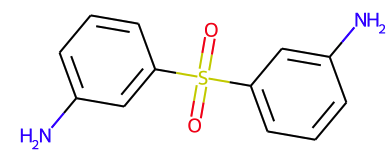
Figure 1 — Representation of a molecule from the dataset
Converting this into a graph consists mainly of representing each atom by a node and replacing the bonds with edges. These nodes and edges are further enriched with various features to avoid losing valuable information such as the name of the atom or the type of bond. In total, input node features are nine-dimensional and edge features three-dimensional.
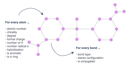
Figure 2— Representation of the molecule as a graph
What are the node features?
- Atomic number: Number of protons in the nucleus of an atom. It’s characteristic of a chemical element and determines its place in the periodic table.
- Chirality: A molecule is chiral if it is distinguishable from its mirror image by any combination of rotations, translations, and some conformational changes. Different types of chirality exist depending on the molecule and the arrangement of the atoms.
- Degree: Number of directly-bonded neighbors of the atom.
- Formal charge: Charge assigned to an atom. It reflects the electron count associated with the atom compared to the isolated neutral atom.
- Number of H: Total number of hydrogen atoms on the atom.
- Number of radical e: Number of unpaired electrons of the atom.
- Hybridization: Atom’s hybridization.
- Is aromatic: Whether it is included in a cyclic structure with pi bonds. This type of structure tends to be very stable in comparison with other geometric arrangements of the same atoms.
- Is in ring: Whether it is included in a ring (a simple cycle of atoms and bonds in a molecule).
Edge features:
- Bond type: Whether the bond is single, double, triple, or aromatic.
- Stereo configuration of the bond.
- Is conjugated: Whether or not the bond is considered to be conjugated.
1.2. What’s Our Target?
The dataset contains the outcomes of 12 different toxicological experiments in the form of binary labels (active/inactive).
The data, as it is, poses two main challenges:
- Small dataset: The number of labeled molecules varies depending on the experiment.
- Unbalanced targets: The percentage of active molecules is very low, up to 3% as shown in the figure below.
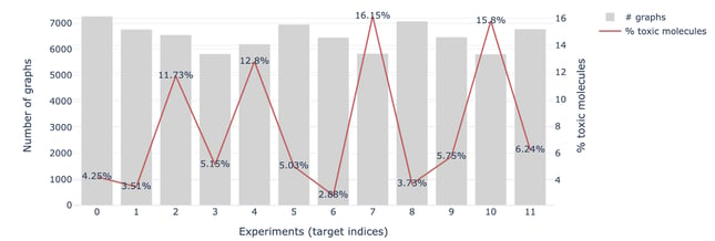
Figure 3 — Number of labeled graphs and percentage of positive outcomes for each experiment
2. GNN for Graph Classification: How Does It Work?
Before diving into how GNN works for graph classification, here is a refresher on the three different types of supervised tasks for graph-based models.
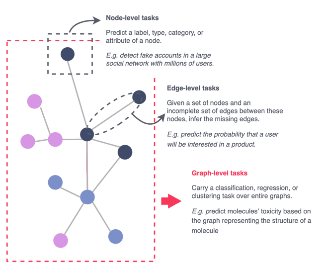
Figure 4 — The different supervised tasks for graph data, illustration by Lina Faik
2.1. The GNN Approach
So far, we have seen in the previous articles of the series that GNNs are able to classify nodes or predict links within a network by learning an embedding of nodes. These embeddings are low-dimensional vectors that summarize the position of nodes in the network as well as the structure of their local neighborhood.
How can this approach be extended to classify whole graphs and not just nodes?
The idea remains the same: GNNs learn to embed entire graphs based on the structural properties of these graphs.
Learning From Multiple Graphs at Once
As graphs tend to be small, it’s better to use batches of graphs instead of individual graphs before inputting them into a GNN.
In NLP or computer vision, this is typically done by rescaling or padding each element into a set of equally-sized shapes. For graphs, those approaches are not feasible. Instead, we can:
- Stack adjacency matrices in a diagonal manner leading to a large graph with multiple isolated subgraphs.
- Concatenate node features and the target.
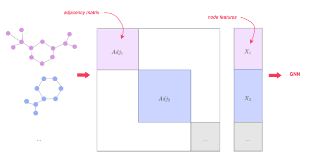
Figure 5 —Mini-batching of graphs, illustration by Lina Faik, inspired by [2]
This approach is the one implemented in PyTorch. It has two main advantages:
- It does not require changing GNN operators using a message passing scheme as, by construction, messages are not exchanged between two nodes of different graphs.
- There is no risk of having a computational or memory overload since the adjacency matrices are saved sparsely (only the non-zero entries which correspond to the edges are kept).
Model Architecture
The model learns to classify graphs using three main steps:
- Embed nodes using several rounds of message passing.
- Aggregate these node embeddings into a single graph embedding (called readout layer). In the code below, the average of node embeddings is used (global mean pool).
- Train a classifier based on graph embeddings.
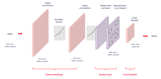
Figure 6 — GNN model architecture, illustration by Lina Faik
You can find below the code used.
What About Edge Features?
The type of bond that links two atoms in a given molecule holds valuable information about the molecule such as its stability, its reactivity, the presence of some chemically organic functional groups, etc. Therefore, including this feature has the potential to improve model performance.
But how can edge features be used when training the model?
If we take the example of GCN, it can easily be done by replacing the zeros and ones of the adjacency matrix with the edge weights, as illustrated in Figure 7. In this context, each message-passing iteration through the GCN updates the hidden embedding of nodes based on the aggregated and now weighted information of their neighborhood.
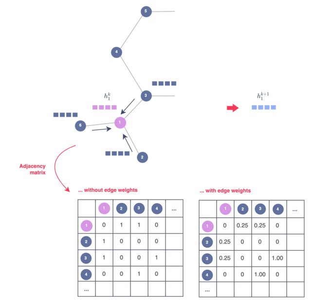
Figure 7 — Including edge weights in a GNN model via the adjacency matrix, illustration by Lina Faik
Other more sophisticated approaches to include the weights or categorical features of features exist. For more information, you can watch this short video here from DeepFindr which gives a large overview of the possibilities.
2.2. Application to the Detection of Toxic Molecules
Methodology
Target. As seen in the first section, the molecules are labeled depending on the experiment. For this reason, each experiment outcome is taken as an individual classification task.
Train / Test sets. The data is divided into two datasets: a training set, which contains around 70% of the total number of graphs, and a test set that contains the rest of the graph. This split is randomly done three times for each model.
Model evaluation. The models are trained using cross-entropy loss with class weights. They are evaluated according to the mean accuracy measured on the test sets, as well as other common classification metrics.
Hyperparameters. For each target, multiple parameters are tested such as the type and number of GNN convolutions used for node embedding (e.g., GCN, GAT, etc.), the latent dimension of node embedding, and the learning rate.
Features. Node features are all used when training the model. Concerning the edge features, the possibility of using the type of bonds (single, double, or triple) was also tested.
Results
The results show satisfactory accuracy on average. However, the accuracy depends to a large extent on the number of labeled molecules (the higher the better) and the percentage of positive outcomes (the lower the worse).
As for the hyperparameters, the best combination also differs depending on the target. Hence, it is difficult to draw a general rule.
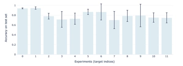
Figure 8 — Accuracy of models on test set depending on the target (experiment)
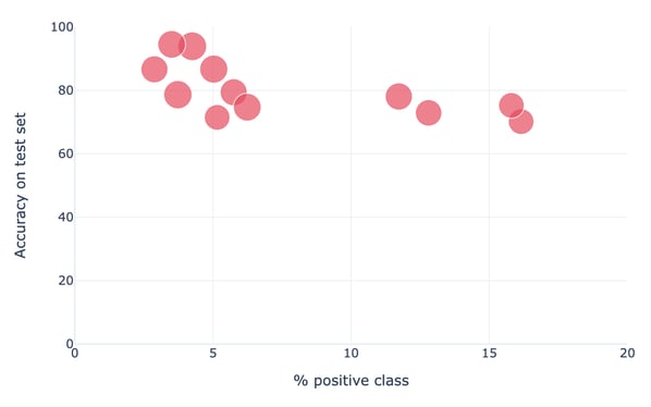
Figure 9 — Accuracy of models on test set vs. % positive class, a large dot size means a high number of labeled graphs for the experiment
3. What About Explainability for GNN?
3.1. A Quick Overview of Approaches
Getting good performance is one thing, but having confidence in the prediction to take action is another. To trust the prediction of a model, one can examine the reasons why the model generated it. Sometimes, these explanations can be more important than the results themselves as they reveal the hidden patterns that the model has detected and better guide the decision-making.
For graphs, explicability is about three questions:
- Which nodes and features were relevant to making the prediction?
- How relevant were they?
- How relevant were the node and edge features of the graph?
What approaches are used to answer these questions?
The paper [5] contains a survey of current methods of GNN explicability. It classifies them in this tree which gives a good overview of the different types of approaches.
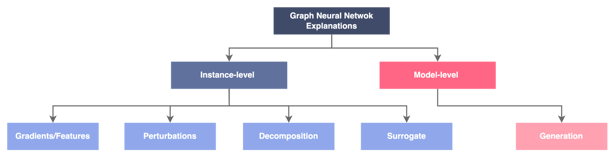
Figure 10 — Classification of the explainability approaches for graphs, illustration by Lina Faik, inspired by [5]
First, it is important to distinguish between:
- Instance-level methods, that provide explanations at the level of individual predictions
- Model-level approaches, that give explanations at the level of the whole model
Let’s explore explanations at the instance level:
- Gradient or features-based methods: They rely on the gradients or hidden feature maps to approximate input importance. Gradients-based approaches compute the gradients of target prediction with respect to input features by back-propagation whereas feature-based methods map the hidden features to the input space via interpolation to measure importance scores. In this context, larger gradients or feature values mean higher importance.
- Perturbation-based methods: They examine the variation in the model predictions with respect to different input perturbations. This is done by masking nodes or edges and observing the results for instance. Intuitively, predictions remain the same when important input information is kept.
- Decomposition methods: They decompose prediction into the input space. Layer by layer the output is transferred back until the input layer is reached. The values then indicate which of the inputs had the highest importance on the outputs.
- Surrogate: Train a simple and interpretable surrogate model to approximate the predictions of the model in the neighboring area of the input.
3.2. Application of GNNExplainer to the Use Case
GNNExplainer falls into the category of perturbation-based methods.
Without going into technical details, it basically consists of learning soft masks for edges and node features. To do so, it starts by randomly initializing soft masks and combining them with the original graph via element-wise multiplications. Then, the masks are optimized by maximizing the mutual information between the predictions of the original graph and the predictions of the newly obtained graph.
More information is available in the original paper [6].
Figure 11 shows the explanations obtained for a molecule of the test set. The more the links between the atoms tend towards the red, the more they played an important role in the prediction.
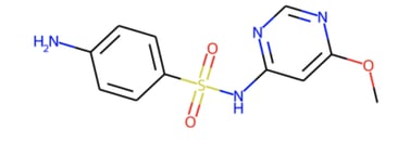
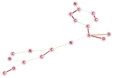
Figure 11 — Explanations obtained for a given prediction using GNNExplainer
Strong knowledge of organic chemistry is needed to investigate the consistency of the results. However, one might note that the presence of SO2 was detected as important. This is the formula of sulfur dioxide which is a chemical compound known to be toxic.
4. Key Takeaways
✔ Graph Neural Networks, GNNs, can be used to classify entire graphs. The idea is similar to node classification or link prediction: learning an embedding of graphs (instead of nodes) using the structural properties of these graphs.
✔ When it comes to understanding the outcome of a model for a given instance, many approaches exist. They can rely on the gradient or features, use perturbation techniques, decompose the outcome, or use surrogate models.
✔ ️The real-life applications are multiple. This article was about the detection of the toxicity of molecules. Predicting other molecular properties lends itself well to this graph-based approach.
✔ ️However, biology is not the only industry. It can be used for instance in the retail industry: this article explains how GNNs can be applied to generate recommendations based on the graph of users’ sessions.
References
[1] M.S. Attene-Ramos et al., Encyclopedia of Toxicology (Third Edition), 2014
[2] Pytorch Geometric tutorials, Graph Classification
[3] Tong Ying Shun, John S. Lazo, Elizabeth R. Sharlow, Paul A. Johnston, Identifying Actives from HTS Data Sets: Practical Approaches for the Selection of an Appropriate HTS Data-Processing Method and Quality Control Review. J. Biomol. Screen. 2010
[4] Evan N. Feinberg, et al, MoleculeNet: A Benchmark for Molecular Machine Learning, Zhenqin Wu, Bharath Ramsundar, March 2017
[5] Hao Yuan, Haiyang Yu, Shurui Gui, Shuiwang Ji, Explainability in Graph Neural Networks: A Taxonomic Survey, December 2020
[6] Rex Ying, Dylan Bourgeois, Jiaxuan You, Marinka Zitnik, Jure Leskovec, GNNExplainer: Generating Explanations for Graph Neural Networks, March 2019
[7] CS224W: Machine Learning with Graphs, Stanford
Thanks to Léo Dreyfus-Schmidt