For the summer, Dataiku integrated me into their fantastic data science team. I hit the ground running, working on a $10,000 data-for-good competition with three colleagues - and we won 3rd prize! Here, I'll share the methodology that (nearly) won this data science competition.
The Competition
Last month, my 83-year-old grandfather tripped over a radio cable in the middle of his living room. He found himself lying on his injured back. Unable to reach for the phone, he stayed there for two days. If it was not for his caring neighbors, worried that they hadn't seen him in a while, this story might well have had a different outcome.
The Safe Aging SPHERE research project has been launched to prevent such dramatic situations. Its purpose is to help the elderly – like my grandfather – safely live at home while maintaining their privacy and independence. Using passive and non-intrusive monitoring, they infer the individual's current activity. If an anomalous activity is detected, then his family or doctor are alerted.
Sounds great, but what does that have to do with data science? Well, machine learning might help to infer a person's current activity based on monitoring.
The Safe Aging with SPHERE project thus asked DrivenData to hold a two-month competition. More than 500 data scientists implemented their best activity-recognition models. The goal was to predict, on a second-by-second basis, 1 of 20 different predefined activities the person may be performing: sitting, lying, walking, ascending stairs, etc. The three most efficient models shared a prize of $10,000.
"Hiding within those mounds of data is knowledge that could change the life
of a patient, or change the world."
Atul Butte, Stanford University
Raw, Noisy, And Hard-To-Interpret Data
Let's start with the basics: the raw data. For this contest, the SPHERE team equipped a house with three sensor modalities:
-
Accelerometers: Participants wore a tri-axial accelerometer on their dominant wrist. The device wirelessly transmits the value of acceleration to several receivers positioned within the house. It gives two valuable pieces of information. First, the value of acceleration in three directions. Second, the signal power that was recorded by each receiver (in units of dBm) - which will be informative for indoor localization.
-
Cameras: Three cameras were used in the living room, hallway and kitchen. In order to preserve the anonymity of the participants, the raw video data is not shared. Instead, the coordinates of the individual’s bounding box and centre of mass are provided.
-
Environmental Sensors: The values of passive IR sensors are given.
Interestingly, the train and test sets were inherently different.

In order to generate the train data, 10 participants successively performed a script of daily-life actions in this house. Hence, the train data consists of 10 continuous sequences of monitoring. Each sequence was recorded on a second-by-second basis and lasts approximately 30 minutes.
The test data was generated by 10 other participants who followed the same script of daily-life actions. So, these 10 test sequences of monitoring were also recorded on a second-by-second basis and have a similar duration. However, instead of supplying 10 continuous test sequences of 30 minutes of monitoring, the SPHERE team randomly SPLIT them into 800 smaller subsequences. To do so, they iteratively sampled a subsequence duration and a number of seconds to drop between two subsequences. The subsequence duration was chosen to follow a uniform distribution between 10 and 30 seconds. The gap length follows a similar distribution.
This was probably done so that we cannot use the script to predict an individual’s activity - the machine learning models would have to generalize to other scripts and participants, making them reusable in real-life situations.
Make the Train And Test Sets Look Alike
Given this challenge, the first step was to change the structure of the train set to have it look like the test set. Therefore, we randomly sampled the 10 train sequences of 30 minutes to 800 smaller subsequences of 10 to 30 seconds, to follow the test set creation methodology.
By doing this random splitting several times with different random seeds, it is possible to generate many train sets. Then, we could follow a bagging approach: create one model per train set and average their predictions. This approach showed good results in cross validation, but, due to time constraint, it was not part of our final model.
Find a Robust Cross-Validation Strategy
Proper cross-validation is needed to estimate the performance of our models and to avoid overfitting. Train and test sets were generated with two distinct groups of individuals. We wanted our cross-validation strategy to reflect this fundamental property. So we divided our train set into a train subset and a validation subset in the following way: data generated by users 6 and 10 formed the validation subset; the 8 remaining users formed the train subset.
We observed for each model a gap between our cross-validation score and that of public leaderboard. However, every improvement in our local cross-validation score led to a similar improvement on public leaderboard.
Note that this strategy might not be optimal. It might even cause overfitting if users 6 and 10 – who form the validation subset and who were chosen for early stopping for XGBoost grid search parameters – turn out to be more similar to the users involved in public leaderboard than to those involved in private leaderboard!
Feature Engineering
Feature engineering aims at converting raw, hard-to-interpret variables into meaningful ones. This step is key in many machine learning problems since it can determine the quality of predictions. First, we computed some basic features: speeds, accelerations, rotations, etc. They should intuitively help us predict the activity performed by the individual.
Second, we added lags on most variables. How? By adding features that inform on the value of each variable 1 second ago, 2 seconds ago, and up to 10 seconds ago. Note how crucial it is to make train and test sets look alike. In the test set, lagged values are always empty for the first line of each subsequence. Whereas for the train set, if we had not split train data into subsequences, lagged values would hardly be empty. Homogenizing the structure of both sets enabled the lag variables to have similar distributions for both sets - we therefore avoided a covariate shift.
After a while, we realized that our feature engineering was way too honest! Since adding lags worked well, why couldn't we add reverse lags? Reverse lags – or leads – turned out to add a lot of information resulting in significant cross-validation score improvements. Now, you might wonder whether or not we should use reverse lags in real-life applications? For instance, if someone has a problem (fainting…), should we really wait before sending an ambulance in order to add reverse lags to our predictive model and be sure that he indeed has a problem ? Well, since 10 seconds is quite short compared to the time it takes to send an ambulance, our gut feeling is that waiting 10 seconds for reverse lags, before taking the decision to send an ambulance, might turn out to be worthwhile.
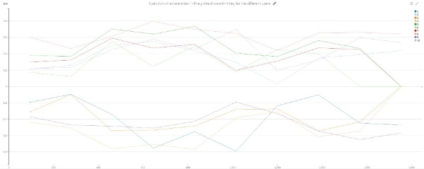
Fun fact: Since the accelerometer was fixed on the individual's dominant wrist, we noticed that two distributions coexisted in the acceleration data: one for right-handed individuals and another one for left-handed ones. To correct this bias, we multiplied accelerometer x and y data by -1 for left-handed individuals.

The evolution of y-acceleration over time suggests that two distributions coexist in acceleration data.
Enriching the Data With Stack Transferring!
Ever wondered how to use a variable that is present in the train set, but absent in the test set? Well, here's a clever and performant concept that you might have been looking for! We call it stack transferring. Let's take a look at an example.
In our competition, a room variable indicates the room where the individual is located. Intuitively, this variable should be very useful to predict the activity of the person: for instance, when someone is in the toilet, it should be very improbable for him to be jumping or lying down! Unfortunately, this room variable is available in the train set, but it is missing in the test set. Here's the stack transferring techniqu, to deal with such variables. It consists of three steps.
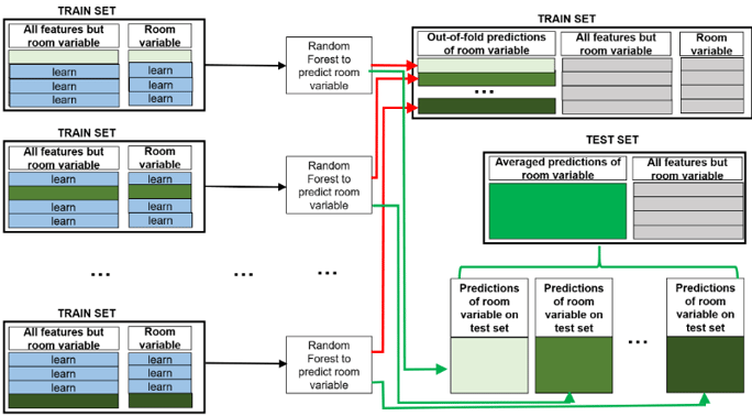
On the train set, update the room variable: replace its exact values by its out-of-fold predictions
On the train set, you should replace the exact values of the room variable by out-of-folds predictions of the room variable. In other words, use 9 folds of the train set - corresponding to 9 participants out of 10 - to predict the room variable on the remaining fold. By doing so 10 times, you can predict the room variable on all the train set!
Now, you can update the room variable on the train set: drop the exact values of the room variable and keep its out-of-fold predictions.
On the test set, predict the room variable
The room variable is missing on the test set. No matter, you can add it to the test set by predicting it! In step 1, you have trained 10 models that predict the room variable. Simply apply them to the test set and average their predictions. Now, the room variable should be available on the test set.

Steps 1 and 2 of stack transferring. 10 models have been used to compute out-of-fold predictions of the room variable on the train set (red arrows). The 10 models were then used to predict the room variable on the test set (green arrows).
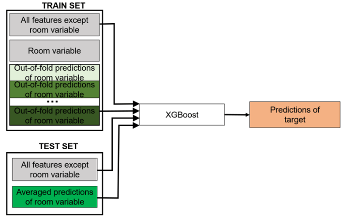
Use the out-of-folds predictions of the room variable to predict the activity variable
Now that you have updated the room variable on the train set, and now that you have predictions of the room variable on the test set, you can add this variable to the model. It should improve the activity prediction!
Notice that the individuals of train and test sets were asked to perform the same list of actions in the same order. Therefore, the room variable had the same distribution on train and test sets. This is a necessary condition if you want stack transferring to perform well.

Step 3 of stack transferring. The (out-of-fold) predictions of room variable are used to predict the target variable on the test set
Fine-Tune Individual Models to Enter Top 5, Stack to Take the Lead
So, to what extent did feature engineering improve our predictions?
It's in general a good idea to start with a simple model that does not need much tuning – like random forests – while you are doing feature engineering. They are easy to implement and able to handle large amounts of variables, so they give you valuable feedback on the quality of your work. Feature engineering diminished our random forest's error-rate from 22% to 16.4%, ranking us 15th of the competition.
When performance seems to reach a plateau even when you are adding new features, try other models that require more tuning. We then went on for the machine learning blockbuster – XGBoost. Once fine-tuned, it performed very well, decreasing our error rate to 14.6% and ranking us top 5!
Finally, we decided to give the stacking technique a try. This ensemble learning technique combines the predictions of diverse individual models and leverages their strengths. Stacking 10 individual models – including linear regressions, Naive Bayes classifiers, random forests, extra-trees and XGBoost models – turned out to perform well, reducing our error rate to 12.9% and ranking us number 1 at that point!

The Flow of our Final Model
Goodies: What We Tried That Did Not Work
From then on, our efforts aimed to maintain our first position. Here are a couple of clever ideas that were not fully implemented.
"Success consists of going from failure to failure without loss of enthusiasm."
Sir Winston Lenoard Spencer-Churchill
Customize XGBoost to directly optimize the brier score
A promising idea was to customize the XGBoost classifier, so that it optimizes predictions for the competition's metric – the Brier score.
Doing so turned out to be trickier than expected. Indeed, XGBoost provides a Python API to customize loss functions for regression and binary classification, but unfortunately not for multi-class classification or multi-dimensional regression. After a bit of math, we managed to implement the gradient and an approximation of the hessian functions of the Brier score directly in the C++ XGBoost source code – it compiled and worked well! This custom XGBoost reached a slightly better cross-validation score than the traditional XGBoost. Unfortunately, we were not able to integrate its predictions to the final model, due to time constraints.
Post-processing
Imagine that someone is lying on a bed at a given moment. You might agree that it is rather probable for him to still be lying the next second, but rather improbable for him to be jumping the next second, right? In other words, each transition, from one activity to another, has a certain probability, which can be high or low. This mathematical property is known as the Markov chain property. A great way to take advantage of this underlying structure is to implement Hidden Markov Models. Yet, given the deadline, we rather opted for a post-processing that smooths predictions. We averaged each prediction with that of the previous and following seconds.
Fun fact: We tried to implement post-processing a couple of hours before the end of the competition. We struggled with the indexes of the different datasets and eventually managed to implement the post-processing at 11:57 pm. Post-processing gave tremendous cross-validation results. But uploading this result took 3 minutes: it was 12:00 pm, and the competition had come to an end without taking into account our promising post-processing!
Wait For The Results
Since we were not able to submit our last-minute post-processing, which might have secured the first position, we felt a bit feverish. A couple of minutes after the deadline, private leaderboard results were announced: we were awarded 3rd prize!

Overall, this data-for-good challenge was a thrilling experience! Diminishing the Brier score from 0.33 (naive prediction) to 0.129 (best model) enabled me to learn a lot in terms of machine learning techniques, methodology and team work. I hope that our work for the competition will help easing the aging process for seniors like my grandfather. Thank you Safe Aging with SPHERE and DrivenData for holding this exciting competition!


