


We often talk about machine learning in the context of predictive analysis and AI. Machine learning is, more or less, a way for computers to learn things without being specifically programmed. But how does that actually happen?
The answer is AI algorithms. AI algorithms are sets of rules that a computer is able to follow. Think about how you learned to do long division — maybe you learned to take the denominator and divide it into the first digits of the numerator, then subtract the subtotal and continue with the next digits until you were left with a remainder. Well, that’s an AI algorithm, and it’s the sort of thing we can program into a computer, which can perform these sorts of calculations much, much faster than we can.


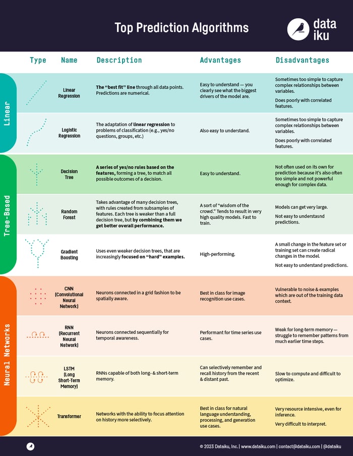
In the latest article of our "In Plain English" blog series, we've put together a brief summary of the top AI algorithms used in predictive analysis, which you can see just below. Read on for more detail on these AI algorithms.
What Does Machine Learning Look Like?
In machine learning, our goal is either prediction or clustering. Today, we’re going to focus on prediction (we’ll cover clustering in a future article). Prediction is a process where, from a set of input variables, we estimate the value of an output variable. For example, using a set of characteristics of a house, we can predict its sale price. Prediction problems are divided into two main categories:
- Regression problems, where the variable to predict is numerical (e.g., the price of a house)
- Classification problems, where the variable to predict is part of one of some number of predefined categories, which can be as simple as "yes" or "no," such as predicting whether a certain piece of equipment will experience a mechanical failure
With that in mind, today we’re not going to reveal a secret to do prediction better than the computers, or even how to be a data scientist! What we are going to do is introduce the most prominent and common AI algorithms used in machine learning historically and today.
These algorithms come in three groups: linear models, tree-based models, and neural networks.
Linear Model Approach
A linear model uses a simple formula to find the “best fit” line through a set of data points. This methodology dates back over 200 years, and it has been used widely throughout statistics and machine learning. It is useful for statistics because of its simplicity — the variable you want to predict (the dependent variable) is represented as an equation of variables you know (independent variables), and so prediction is just a matter of inputting the independent variables and having the equation spit out the answer.
For example, you might want to know how long it will take to bake a cake, and your regression analysis might yield an equation t = 0.5x + 0.25y, where t is the baking time in hours, x is the weight of the cake batter in kg, and y is a variable which is 1 if it is chocolate and 0 if it is not. If you have 1 kg of chocolate cake batter (we love cake), then you plug your variables into our equation, and you get t = (0.5 x 1) + (0.25 x 1) = 0.75 hours, or 45 minutes.
Linear Regression
Linear regression, or more specifically “least squares regression,” is the most standard form of linear model. For regression problems, linear regression is the most simple linear model. Its drawback is that there is a tendency for the model to “overfit” — that is, for the model to adapt too exactly to the data on which it has been trained at the expense of the ability to generalize to previously unseen data. For this reason, linear regression (along with logistic regression, which we’ll get to in a second) in machine learning is often “regularized,” which means the model has certain penalties to prevent overfit.
Another drawback of linear models is that, since they’re so simple, they tend to have trouble predicting more complex behaviors when the input variables are not independent.
Logistic Regression
Logistic regression is simply the adaptation of linear regression to classification problems (once again, discussed above). The drawbacks of logistic regression are the same as those of linear regression. Because it maps values between 0 and 1, it is suited for classification problems as it can represent the probabilities of being in each class.
Tree-Based Model Approach
When you hear tree-based, think decision trees, i.e., a sequence of branching operations.
Decision Tree
A decision tree is a graph that uses a branching method to show each possible outcome of a decision. Like if you’re ordering a salad, you first decide the type of lettuce, then the toppings, then the dressing. We can represent all possible outcomes in a decision tree. In machine learning, the branches used are binary yes/no answers.
To train a decision tree, we take the train dataset (that is, the dataset that we use to train the model) and find which attribute best “splits” the train set with regards to the target. For example, in a fraud detection case, we could find that the attribute which best predicts the risk of fraud is the country. After this first split, we have two subsets which are the best at predicting if we only know that first attribute. Then we can iterate on the second-best attribute for each subset and re-split each subset, continuing until we have used enough of the attributes to satisfy our needs.
Random Forest
A random forest is the average of many decision trees, each of which is trained with a random sample of the data. Each single tree in the forest is weaker than a full decision tree, but by putting them all together, we get better overall performance thanks to diversity.
Random forest is a very popular AI algorithm in machine learning today. It is very easy to train, and it tends to perform quite well. Its downside is that it can be slow to output predictions relative to other AI algorithms, so you might not use it when you need lightning-fast predictions.
Gradient Boosting
Gradient boosting, like random forest, is also made from “weak” decision trees. The big difference is that in gradient boosting, the trees are trained one after another. Each subsequent tree is trained primarily with data that had been incorrectly predicted by previous trees. This allows gradient boost to gradually focus less on the easy-to-predict cases and more on difficult cases.
Gradient boosting performs very well. However, small changes in the training dataset can create radical changes in the model, so it may not produce the most explainable results.
Neural Networks
Neural networks refer to a biological phenomenon of interconnected neurons that exchange messages with each other. This idea has now been adapted to the world of machine learning and is called ANN (Artificial Neural Networks). Deep learning, which you’ve heard a lot about, can be done with several layers of neural networks put one after the other.
ANNs are a family of models that are taught to adopt cognitive skills. No other algorithms can handle extremely complex tasks, such as image recognition, as well as neural networks. However, just like the human brain, it takes a very long time to train the model, and it requires a lot of power (just think about how much we eat to keep our brains working!).
Convolutional Neural Networks
CNNs are comprised of neuron layers connected in a lattice pattern. These grid-like structures are effective at learning spatial relationships, which is particularly useful when working with imagery. Earlier layers capture a sense of edges, color, light, and shadow, whilst latter layers aggregate upon earlier characteristics to represent features more recognizable in nature, such as faces.
Recurrent Neural Networks
RNNs contain neurons connected to themselves over sequential time steps, meaning that the weights are determined not only by the current input example, but also those which were recently seen by the same neuron. This is helpful for representing temporal relationships as the model maintains a sense of history whilst learning the patterns behind the data.
Long Short-Term Memory Networks
LSTMs are a type of RNN which introduce a notion of selective memory, enabling the network to hold information received earlier in a sequence, for a much longer number of steps than ordinary RNNs, when required. This is helpful when modeling seasonal behavior with large periodicities.
Transformers
Transformers go beyond RNNs and LSTMs by treating sequences of input together at one instance, rather than sequentially, “paying attention” to each part of the input sequence in the context of other elements, to understand which elements are more strongly related to each other than others. This design allows the network to be trained and executed in a parallelized manner.