


In this series of blog posts, we have been exploring the problem of augmenting a table using information contained in a data lake (a large collection of datasets). First, we explored how to combine tables through intelligent join suggestion, then we considered how to scale the problem through set matching with hash-based methods.
Here, we continue our discussion by evaluating how some of the strategies described in the previous posts perform in a realistic scenario: We seek to evaluate how potential joins augment a “base table” by measuring how retrieving and selecting the correct candidates improves the performance of a downstream machine learning (ML) task.
In our scenario, we build a pipeline that breaks down into four tasks spread across three steps: retrieving the join candidates, selecting which candidates should be merged with the base table (this join step combines merging and aggregation) and, finally, training an ML model on the joined table to predict the target variable.
Retrieving Candidates
The first task focuses on identifying those tables that can be joined exactly with the base table. As exact joins on keys are functionally set intersections, we use Jaccard Containment (JC) as a metric: The containment of a set Q in another set X is the “normalized intersection,” i.e., “How much of Q is contained in X”:

Measuring the intersection gives a good indication of how many of the rows in a given column can be “matched” by rows in a candidate column, and all the retrieval methods we consider do so in some way:
- Exact Matching computes the exact containment between the given query column and all columns in the test data lake.
- MinHash relies on hashing sets to estimate the containment of the query in the data lake (refer to the previous blog post for more detail). MinHash returns all candidates above a defined threshold with no inherent ordering.
- Hybrid MinHash ranks the candidates retrieved by MinHash by measuring their exact containment.
- Starmie (original paper) employs language models to build an embedded representation of the query column and each column in the data lake. The similarity between a candidate column and the query column is then measured by combining containment and semantic similarity.
To aid comparison, we plot the results for each retrieval method relative to the average for all methods. The value is then reported as 1x (or 0%) axis in each plot.
Trading Resources for Performance
Retrieval methods that measure exact set similarity (Exact Matching, Starmie) consistently outperform those that rely on approximate estimations (MinHash, Hybrid MinHash). Hybrid MinHash mitigates the situation, but the performance is still inferior.
Starmie is far more expensive than the alternatives in both peak RAM usage and time required to retrieve candidates, but this larger computational cost does not result in an equivalent gain in the prediction performance.
Scaling With Queries
While this seems to suggest that methods based on exact metrics would be the way to go, it is important to note that these methods scale much worse when the number of query columns increases compared to hash-based methods.
We show this in the figure above: Hash-based methods incur a large initial cost due to having to index the data lake. Conversely, Exact Matching exhibits a steeper slope because measuring the exact containment is a costly operation that must be repeated for every query column. In other words, the more queries you need to run against a static data lake, the more advantageous an index-based solution like MinHash can be.
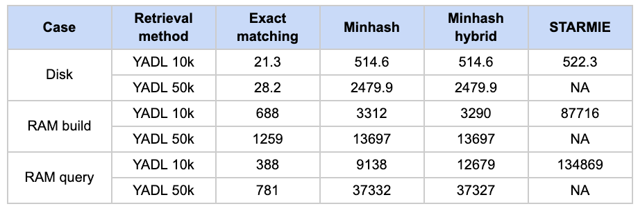
On the RAM and disk usage side, we observe that Exact Matching, in general, has the smallest footprint and RAM usage. MinHash strikes a middle ground between the alternatives in RAM, though it requires more space on disk.
Selecting Candidates
The next step identifies — out of all the candidates chosen by the retrieval methods— those that actually improve the prediction performance if joined. We implement four join selection strategies: Each join selector takes as input the base table and the join candidates prepared by a retrieval method from the previous step. Then, the selected candidates are joined with the base table on the query column and, finally, an ML model is trained on the joined table.
- Highest Containment Join: Compute the Jaccard Containment for each candidate, then select the candidate with the highest containment.
- Best Single Join: For each join candidate, train an ML model on the base table joined with the candidate. Measure the prediction performance on a validation set and choose the candidate with the best performance.
- Full Join: Join all candidates and train an ML model on the result.
- Stepwise Greedy Join: Iterate over each candidate. In each iteration, join a new candidate with the main table and test the prediction performance. If the performance improves, keep the joined table, otherwise drop the candidate.
We plot the performance relative to the mean over all selectors:
We can see that selectors that join multiple candidates at the same time — stepwise greedy and full join — outperform those that join only one candidate. Stepwise greedy is much slower than any of the alternatives, and it does not bring significant improvements in the prediction performance.
Is Containment Enough?
When taking a closer look at containment, we notice that exact methods can retrieve all candidates with high containment (left plot), while candidates produced by MinHash-based methods tend to have a much lower average containment compared to their competitors. The plot on the right shows that there is a positive correlation between high containment and good results: This makes sense since the number of “matched rows” between the base table and any candidate is directly proportional to the containment.
However, while these results seem to suggest that containment alone is good enough to guarantee good results, we observe that this is not the case in practice (as the Highest Containment results attest at the join selector stage).
In fact, scenarios that involve very high redundancy may lead to selecting multiple copies of the same candidate, which may have the same containment. High containment candidates may still introduce features that are not useful for the prediction task. Finally, containment does not track set cardinality: A set {0, 1} will have perfect overlap with another set {0, 1}; joining on such candidates will be useless at best and result in a memory error at worst.
Possible solutions to these problems may include performing a sanity check before joining on perfectly matched sets or profiling and filtering base table and data lake tables to prevent issues (e.g., by avoiding numerical keys, low-cardinality columns, etc.).
The overall message is that, while containment does not guarantee good performance, it’s still correlated with it and is therefore still useful. Redundancy and low-cardinality situations may be mitigated by profiling and filtering the data lake before querying.
Aggregation
In our scenario, we are training an ML model and want to maintain the number of training samples constant. If a join involves one-to-many matches (e.g., join a movie director with all their movies), keeping all matches would increase the number of training samples. To avoid this, duplicate rows should be aggregated.
One simple solution is selecting only the first of each duplicate row (first), or the mean of numerical and mode of categorical features (mean). We consider “first” to be equivalent to “random choice”, since for our data lake samples are ordered randomly. The more sophisticated solution Deep Feature Synthesis (DFS) generates new features such as mean, variance, or count of unique values, for each original feature.
The expectation is that the new features introduced by DFS should improve the performance of the model. However, our results show that DFS is only slightly better than the simpler alternatives. Moreover, DFS is far slower because generating features is an expensive process, and the new features increase the training time.
In general, we observe that aggregation in general is not a big concern, especially when the joins are executed over key-like (i.e., very high cardinality) features. In the vast majority of cases, selecting a value at random from the group has the same result as taking the most frequent values.
ML Model
Results relative to the ML model are not surprising: Catboost outperforms the linear regression model, but is noticeably slower in comparison.
There could be more performance gains with hyperparameter optimization, which we do not use as we were more interested in how each task affected the prediction performance, rather than optimizing the performance to its fullest.
Conclusions
Our key takeaways from this benchmark study are that:
- Retrieving the correct candidates has a large impact on the pipeline, because later steps cannot recover lost candidates and make up for poor retrieval performance.
- If it’s not clear what the query column should be. If many columns should be queried, approximate indices should be used. If few queries are expected, or if the larger computational cost is not problematic, exact methods should be favored instead.
- While Jaccard Containment can be a good indicator of a promising join, additional steps in a data augmentation pipeline are necessary to select the most relevant candidate for the downstream task.
- Complex aggregation is expensive and does not bring large benefits.
This post is adapted from the paper “Retrieve, Merge, Predict: Augmenting Tables with Data Lakes”, available at: https://arxiv.org/abs/2402.06282