


In this rapidly advancing AI world, human computer interactions (HCI) are of extreme importance. We live in a world where Siri and Alexa are physically closer to us than other humans. Soon the world will get more populated with physical and virtual service robots to accomplish tasks that range from caring for the elderly to assessing the effectiveness of your marketing campaign. Understanding human emotions paves the way to understanding people's needs better and, ultimately, providing better service.

Sounds cool! But what can you do after you’ve figured out the emotions?
We can find wide applications of speech emotion recognition in marketing, healthcare, customer satisfaction, gaming experience improvement, social media analysis, stress monitoring, and much more. In this article, we are going to build an AI model which can predict the emotion of the speaker by analyzing the recorded audio clip of the speaker’s voice.
Let’s dig into a sample audio data file.
Transcript: “Kids are talking by the door.” [Emotion: Anger]
The above clip will be the input to our AI model. The model predicts the emotion of the speaker as anger.
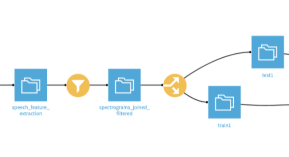
The visualization of the end-to-end flow (the pipeline of the project we are going to build in Dataiku) is below:
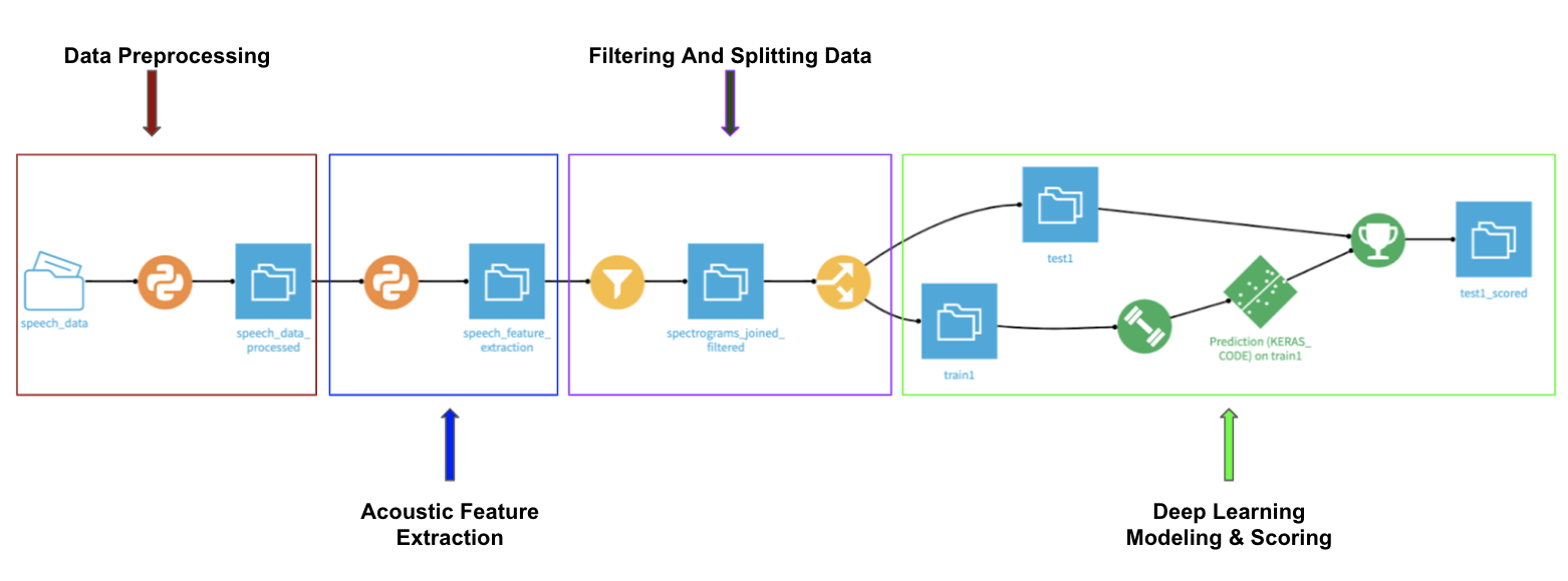
1. Data Processing
So to start, we need audio data of human voices with labeled emotions. We are going to explore a speech emotion recognition database on the Kaggle website named “Speech Emotion Recognition." This dataset is a mix of audio data (.wav files) from four popular speech emotion databases such as Crema, Ravdess, Savee, and Tess. Let’s start by uploading the dataset in Dataiku.
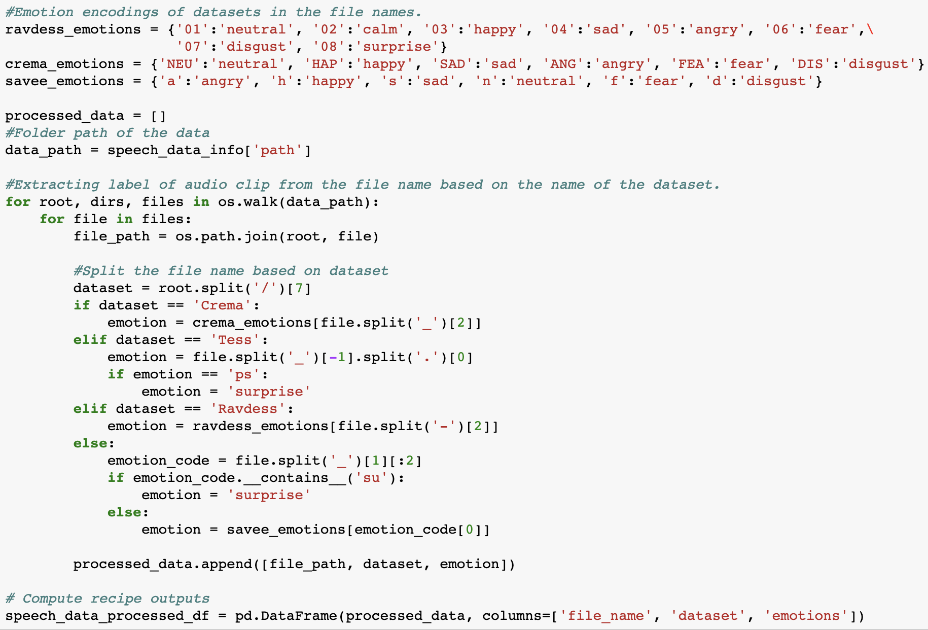
Each audio file in the dataset is embedded with a single emotion. This emotion label can be found as a component in the file name. Therefore, our first step is to extract all the emotion labels of corresponding audio files from their file names. I am using the Python recipe in Dataiku to extract the emotion labels into a desired tabular format.
The code snippet is below:
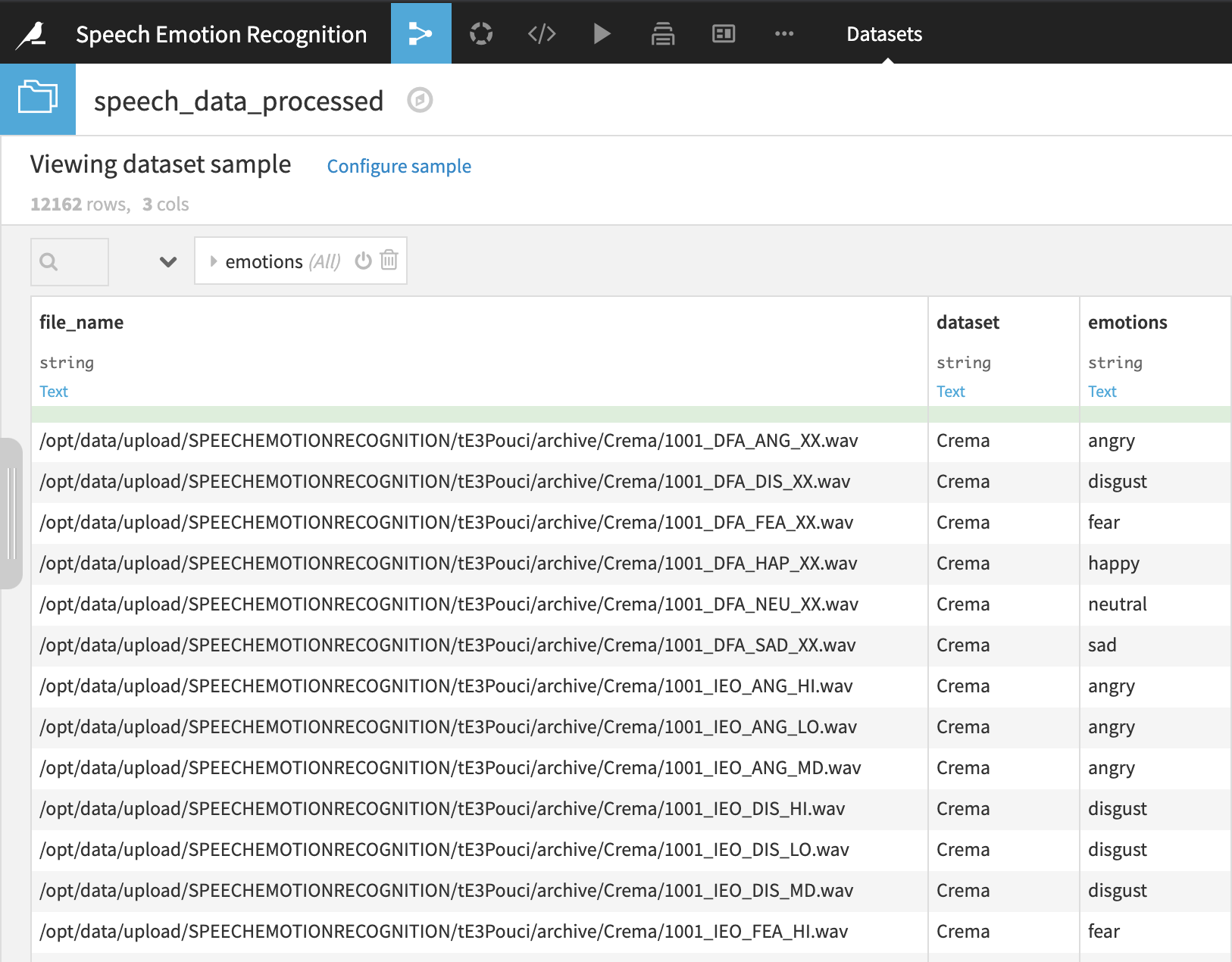
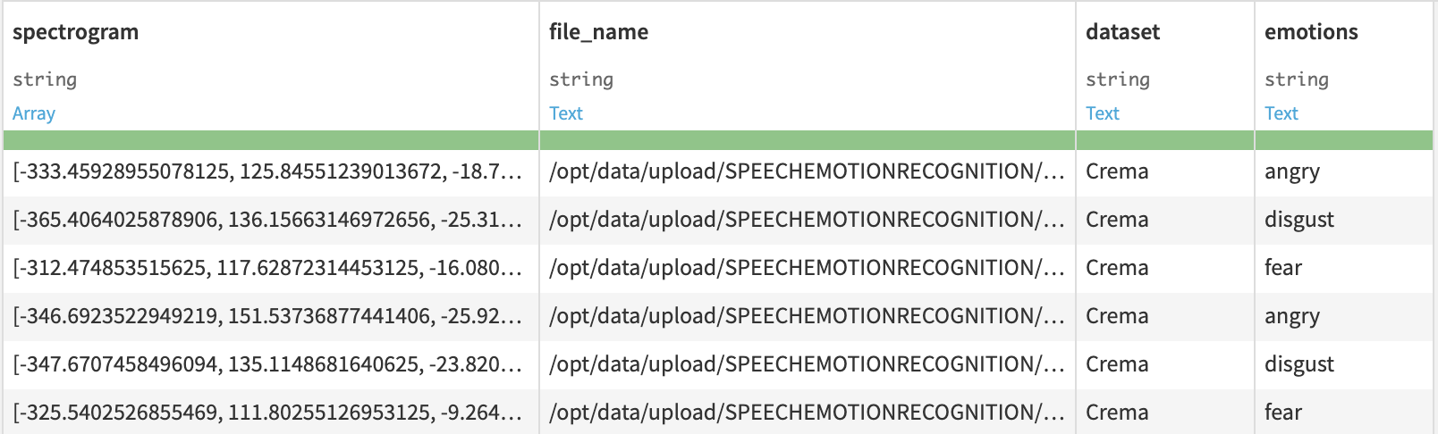
After running the above Python recipe code, the result is a dataset like the below. The file name is the path to the audio file and the dataset is the name of the original dataset (the four popular datasets) it belonged to. Emotions refers to the embedded emotion in the audio clip.
2. Acoustic Feature Extraction
Now we are all set with the audio files and labels. But AI models don't understand anything other than numbers. So the question is: How do we convert an audio file into a numerical representation? The answer is signal processing. Yes, it is time to brace yourself a bit.

How Do We See Sound?
We can see it using the digital representation. The digital representation of an audio clip can be easily obtained by using Python packages such as Librosa, a music and audio analysis package.
Below is the code snippet to read the audio file using Librosa and display the audio as a wave form:
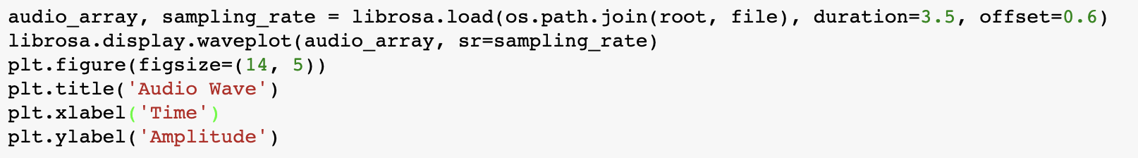
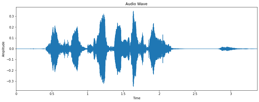
The above plot describes the change in amplitude (loudness) of a signal over time domain. The next challenge is extracting the significant features from this wave form that can easily help to distinguish emotions embedded.
There are numerous ways to extract features from a raw audio waveform using signal processing such as zero crossing rate, spectral centroid, zooming in, and so on. After my experiments, I have decided to move forward with a combination of three main acoustic features which will be discussed below at a high level. In the case of audio waves, the variations in the amplitudes and frequencies contained in it can provide insights. A single audio wave consists of multiple single frequency signals. Extracting these individual, single frequency signals from the audio is called spectrum analysis.
Let’s think about what happens when we hear an audio clip with different kinds of background noise. Human brains are a kind of spectrum analyzer which automatically split up the frequency signals in the audio and help us focus more on the main component, ignoring the single frequency signals of background noise. This same feature of splitting up the single frequencies in an audio file can be obtained by a mathematical technique called Fourier Transform. It basically transforms a time-domain signal into a frequency-domain signal. We now have information on how amplitude and frequency vary with time (separately, not together).
Our next task is to get the frequency and amplitude variations together with time. This is where the Spectogram comes in handy — it is a snapshot of the information of frequency, time, and amplitude in one. We will be using three kinds of spectrograms for our model building as discussed below.
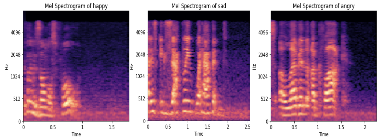
1. Mel Spectogram
It shows how the frequency and amplitude evolve over time. The x-axis represents time, the y-axis represents frequency, and color represents amplitude. The brighter the color, the higher the amplitude. This spectrogram uses a special scale for frequency called the Mel scale. Below are the sample images of the Mel spectrogram of an audio wave with different emotions.

2. Mel-Frequency Cepstral Coefficients (MFCC)
This is one of the most common ways to perform feature extraction from audio waveforms. MFCC features are very efficient in preserving the overall shape of the audio waveform.

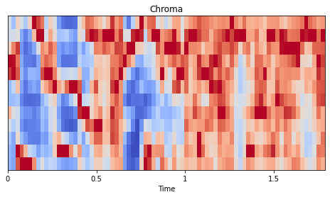
3. Chroma
Chroma is a specific kind of spectrogram based on the chromatic scale. The chromatic scale or 12 tone-scale is a set of 12 pitches used in tonal music.
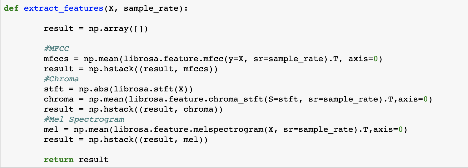
As shown in the above code snippet, an audio file represented by the column mean values of MFCC is stacked horizontally with column mean values of chroma followed by column mean values of Mel Spectrogram. These stacked features will be an array of 268 numbers and are added as a new column named spectrogram.
3. Filtering and Splitting the Dataset
The next step is to explore the underlying emotions of your data. The below histogram depicts the percentage of data that belongs to each class of emotion.
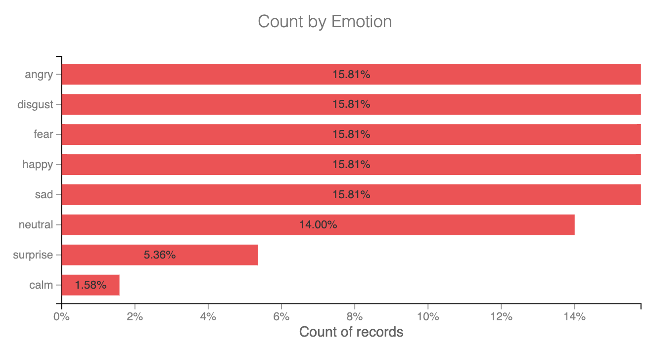
The original dataset has about 12,000 audio files with eight kinds of emotions labeled. The Surprise and Calm emotion class data are comparatively low when compared to others. So, in order to have a balanced dataset, we are going to only focus on the top six emotion classes (disregarding Calm and Surprise classes). The filtering operation is used to filter out all the Calm and Surprise emotion data. This reduced our dataset to around 11,000 audio files.
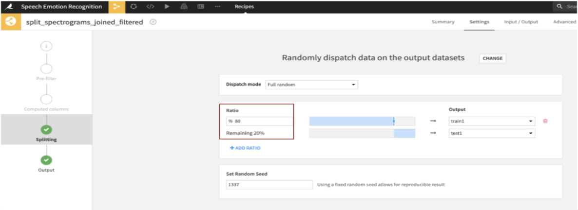
This dataset is further divided into train (80%) and test (20%) data using the split recipe seen below:
4. Acoustic Model Building and Scoring Using Deep Learning

The final step is to build the deep learning model which takes spectrogram features of an audio file as input and predicts the emotion embedded in it. In Dataiku, we can start by creating a new deep learning analysis with the emotions column as the target column.
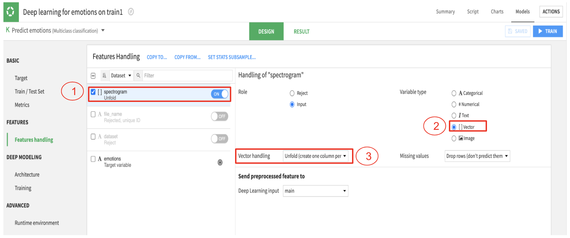
The training dataset is further split into 90% as the training set and 10% as the validation set. The below picture depicts how to choose our spectrogram vector as input to the model. We can toggle on/off to select the features which will be an input to the model in Dataiku. This is particularly useful when you have to run multiple experiments with a subset of features at a time.
Step 1 (as seen in the image below) is to toggle on the spectrogram feature. Our spectrogram feature is an array of numbers which needs to be unfolded before feeding to model. By choosing unfolding options, (Step 2 and 3 in the picture will do this) Dataiku automatically unfolds our data to feed to the network.
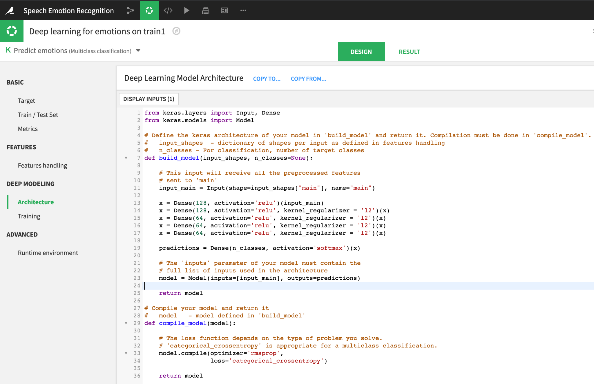
Architecture
I am using Keras library to build my deep neural network architecture — two dense layers of 128 units followed by three dense layers of 64 units and a final layer of six units are used. L2 regularization is added in the last four layers to reduce overfitting.
Training and Validation Accuracy
The model was trained 100 epochs on a batch size of 64. The model obtained a training score of 77% and a validation score of 62%, which suggests that the model is slightly overfit. A test score of 60% was obtained.
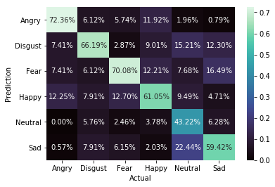
Confusion Matrix of Test Data
These results show that our model can distinguish angry emotions better than other emotions. In the above confusion matrix, we can see 12.25% of Angry emotions get predicted as Happy, which in a way indicates that the model takes the loudness of speech to detect emotion into account. When it comes to Neutral emotion, the model gets confused between Neutral and Sad.
What Next?
There are multiple ways to further improve the accuracy of the model. On the data side, collecting more data and applying augmentation techniques such as adding noise to audio can help to improve the accuracy. On the features part, we can include linguistic features and build new linguistic models along with acoustic models.
This project has a potential to be used in heavy industries such as business process outsourcing (BPO) or call centers. We can improve this project for holistic analysis of call quality and customer experience through following techniques:
- Convert voice to text
- Detect keywords
- Apply topic modeling algorithms such as LDA
With these features, both BPO and call center management can improve their services and their customers will get near real-time feedback from the market through a single platform approach.