Training ML Models With Dataiku and Snowpark ML: A Code Approach

At Dataiku, we’re constantly thinking about building performant, production-ready assets and democratizing data science and AI. 

Two Snowflake offerings align well with these interests:

• Snowpark Python can improve performance — reducing data movement and parallelizing compute (for particular Snowpark APIs, e.g., DataFrames).
• Snowpark ML, Snowflake’s new set of machine learning (ML) tools, makes training ML models easier and more accessible.

We’re particularly excited about the new snowflake-ml-python package, which benefits from running Python code in Snowpark while mirroring the familiar syntax of scikit-learn, XGBoost, and LightGBM that data scientists know and love.

In this blog, we’ll walk through an all-Python-code solution for training models using Dataiku and Snowpark ML.

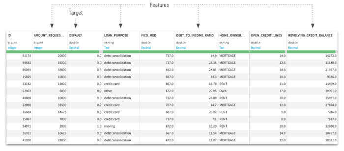
Our use case is predicting loan defaults — we’ll use past known loan data, then train many ML models to predict whether the applicant defaulted or paid back the loan — a two-class classification problem. 

Our models will pick up on the underlying patterns in the data — how our input features relate to our target. Then, we’ll be able to use this model to make (hopefully) accurate predictions for new loan applicants based on their known features.

Here’s our final project flow: 

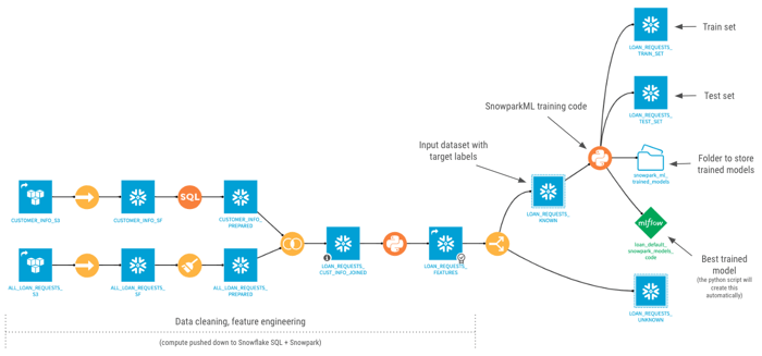
The high-level steps in this project are:

• Connect to past loan request data and customer data in S3
• Sync to Snowflake via fast-path (COPY INTO)
• Clean up messy values with a visual Prepare recipe and custom SQL code
• Join tables together on a shared “CUSTOMER_ID” field
• Engineer new features using Snowpark UDFs

• Process features - rescale, encode, impute for missing values
• Tune hyperparameters for multiple algorithms with a RandomizedSearch
• Deploy the best trained model as a Dataiku Saved Model (green diamond)
• Output trained model artifacts, train, test sets for transparency

We’re going to skip the data cleaning + feature engineering section this time. (If you want to learn more about Dataiku’s data cleaning and feature engineering capabilities specific to Snowflake and Snowpark, check out this video).

Keep reading for a complete step-by-step walkthrough (with code!) on training an ML model with Snowpark ML and Dataiku.

0 - Set Up a Python 3.8 Environment and Python Code Recipe

First, we’ll create a Python 3.8 code environment in Dataiku. We’ve named this one “py_38_snowpark.” Change the core package versions to Pandas 1.3, paste the packages from the list below, then click “Update.”

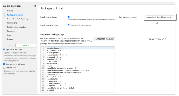
Here’s the full list of packages:

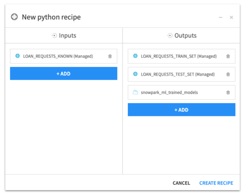
Back to our project flow, we’ll start with a cleaned-up input dataset with labeled target values for all loan applications (default or not). Then, we create a Python recipe with three outputs:

• Train dataset (Snowflake)
• Test dataset (Snowflake)
• Trained model folder (S3)

1 - Import Python Packages 

We start with package imports — you’ll notice the new Snowpark ML Imports toward the bottom. The syntax here is the same as their equivalent classes/functions in scikit-learn, XGBoost, and LightGBM.

2 - Define Recipe Inputs, Outputs, and Other Training Parameters

In this next block of code, we’ll point to our input dataset, two train/test output datasets, and folder to store trained models. We can name our final model, select the target column (in our case, “DEFAULT”), choose the train/test ratio, the scoring metric, whether to use class weights, and other options.

Then, we choose the input features to feed into the model. Note the structure of this list of dictionaries. Each dictionary contains the feature name, the rescaling/encoding method, and missingness imputation method.

3 - Set Up MLflow Experiment Tracking 

MLflow is a great open-source library for tracking ML experiments. Dataiku provides a nice UI on top of MLflow’s experiment tracking functionality. More on that here.

We’ll use the Dataiku and MLflow APIs to create a new experiment to track our model training process.

4 - Set Up the Snowpark Session

Our model training code will run in Snowpark, Snowflake’s runtimes and libraries that deploy and process non-SQL code in Snowflake. Dataiku’s Snowpark integration allows us to create a Snowpark Session using the same credentials we use to connect to the input Snowflake table.

5 - Add a Target Class Weights Column and Split Into Train/Test Sets

We first map the target column data type to a more general type supported by the different ML algorithms.

Then, we add a new “SAMPLE_WEIGHTS” column equal to the class weights of our target column. This will help mitigate target class imbalance problems. Analytics Vidhya has a great explanation of the topic here.

With the standard scikit-learn, XGBoost, and LightGBM algorithm classes, you can simply pass in the class_weights = balanced argument to solve this issue. Snowpark ML doesn’t allow this argument, instead requiring an explicit “SAMPLE_WEIGHTS” column for all rows. The below code block shows how you can do that.

Lastly, we write the train/test Snowpark dataframes as persistent tables in Snowflake.

6 - Create the Feature Transformation Pipeline

Based on the features and preprocessing options we chose earlier, we now translate those into proper Scaler, Encoder, and Imputer classes — then wrap them all into a Pipeline. 

You’ll notice the syntax with these Snowpark ML classes is the same as their scikit-learn equivalents.

7 - Initialize Algorithms and Hyperparameter Spaces for the Randomized Search 

We’re going to try four different algorithms: logistic regression, random forest, XGBoost, and LightGBM. 

We define a hyperparameter search space by passing any parameter we’d like to tune along with the distribution of values to test. 

For example, for the n_estimators parameter, we add a clf__ prefix, then pass a random integer distribution from X to Y. The RandomizedSearch algorithm will randomly try integers between X and Y. 

If you want to try a continuous distribution, you can use something like scipy’s uniform or loguniform (see clf__learning_rate). 

The n_iter parameter controls how many hyperparameter combinations to try for each algorithm.

8 - Train Models, Run Randomized Search

This code runs our model training and hyperparameter tuning process. 

Notice the arguments we pass into the RandomizedSearchCV object: input_cols, label_cols, output_cols, sample_weight_col. These are a bit different than the scikit-learn equivalent, and are fundamental to all ML algorithm classes in the Snowpark ML library. Snowflake explains these differences in their documentation here.

9 - Log Hyperparameters, Performance Metrics, and Trained Model Objects to MLflow

Now that we’ve trained a bunch of models across different algorithms and hyperparameter combinations, let’s track all this information using MLflow.

This code will log the algorithm type, hyperparameters, cross validation performance metrics, and trained model objects (to the S3 folder we chose earlier).

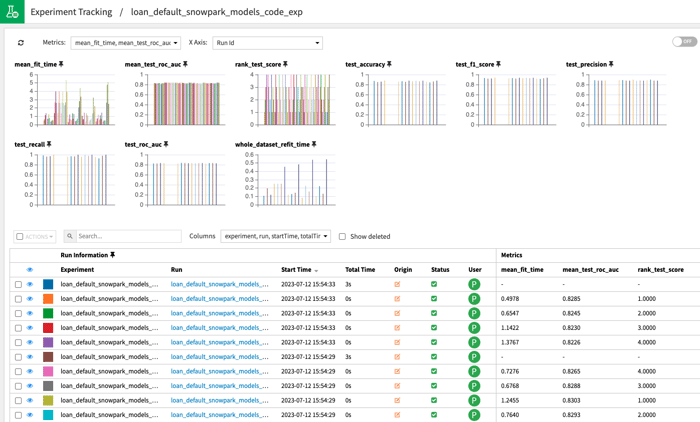
After this code runs, you’ll be able to find all model performance information in Dataiku’s Experiment Tracking tab. Use this tab to diagnose your models, iterate, and improve.

10 - Save the Best Trained Model as a Dataiku Saved Model (Green Diamond) 

This block of code will take the best trained model (according to your chosen performance metric, in our case ROC AUC) and deploy it as a Dataiku Saved Model (the green diamond in our flow).

The last line… 

mlflow_version.evaluate(output_test_dataset_name, container_exec_config_name='NONE')

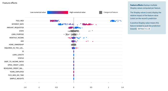
…calculates final model performance on the holdout test dataset. This line also generates Dataiku’s out-of-the-box model performance and explainability charts, like this Shapley feature effects chart:

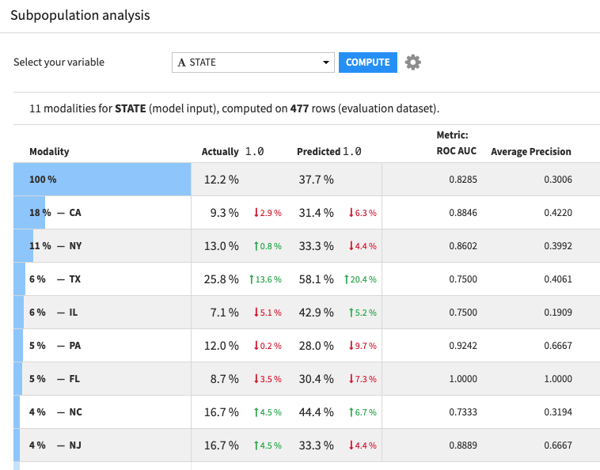
This subpopulation analysis table:

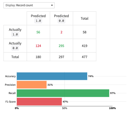
And this confusion matrix:

11 - Add the Dataiku Saved Model as an Output to the Python Recipe

Note: You should only run this last block of code when in the Python recipe itself — don’t run it within a Jupyter notebook. 

This code will add the newly-created Dataiku Saved Model (green diamond) as an output of the Python recipe (rather than it floating in the flow with no input).

What's Next

Congrats! You made it through this dense, code-heavy article. 

From here, we can:

• Create another Python recipe using Snowpark ML for batch inference on new loan applications.
• Deploy the trained model as a RESTful API endpoint for real-time inferencing on Snowpark Container Services, available in Private Preview (video here).
• Use Dataiku's Govern node to control and monitor our deployed models (more on Govern here). 

And of course, feel free to take this framework and example code and apply it to your own use case.