Using Machine Learning to Price Apartment Properties

Moving to a new continent always comes with stressful tasks to complete. One of them is obviously finding your future apartment. This is especially notable in Dubai where real estate pricing is subject to volatility — a volatility that is commonly compared to the stock market’s. Indeed, Dubai is a market of investors and its economy is highly dependent on the oil price.

Recently, some exogenous factors (i.e., end of COVID-19-related lockdowns, the World Expo, the FIFA World Cup hosted in its neighboring Qatar) have influenced/encouraged some landlords to introduce a rise in prices. And when the market gets tight, hunting for an apartment can drive you to overpay for it. 

Finding myself in that exact situation, I decided to build a model that estimates the fair transaction price of apartments for the purpose of preventing overpayment. I had to find a way to derive a fair transaction price for properties to make a wise choice.

There is no universal model for pricing properties, but machine learning is typically a relevant approach. And Dataiku provided me with all the needed capabilities to build such a use case in an easy and intuitive way. This post is intended for data scientists or those who come with a statistical background. We will deal with the case of Dubai, where I moved to. But the modeling approach and usage of Dataiku is somehow agnostic to the underlying data.
It will give an overview on: 

• The methodology followed to model the problem 
• Some modeling challenges faced, which could be the case in many other data science use cases
• Some Dataiku capabilities used for project development (no knowledge of the platform is needed)

At the end, the user will get a project template reusable in a similar context and learn about general modeling approaches and their potential outcome.

Understanding the Data

The data in the use case I will describe comes from a major real estate portal in the United Arab Emirates, which made a subset publicly available. Around 2,000 apartment unit transactions are listed. Each property comes with specific details like:

• Price
• Number of bedrooms 
• Number of bathrooms
• Covered area
• Location details (i.e., area name, latitude, longitude)
• List of amenities

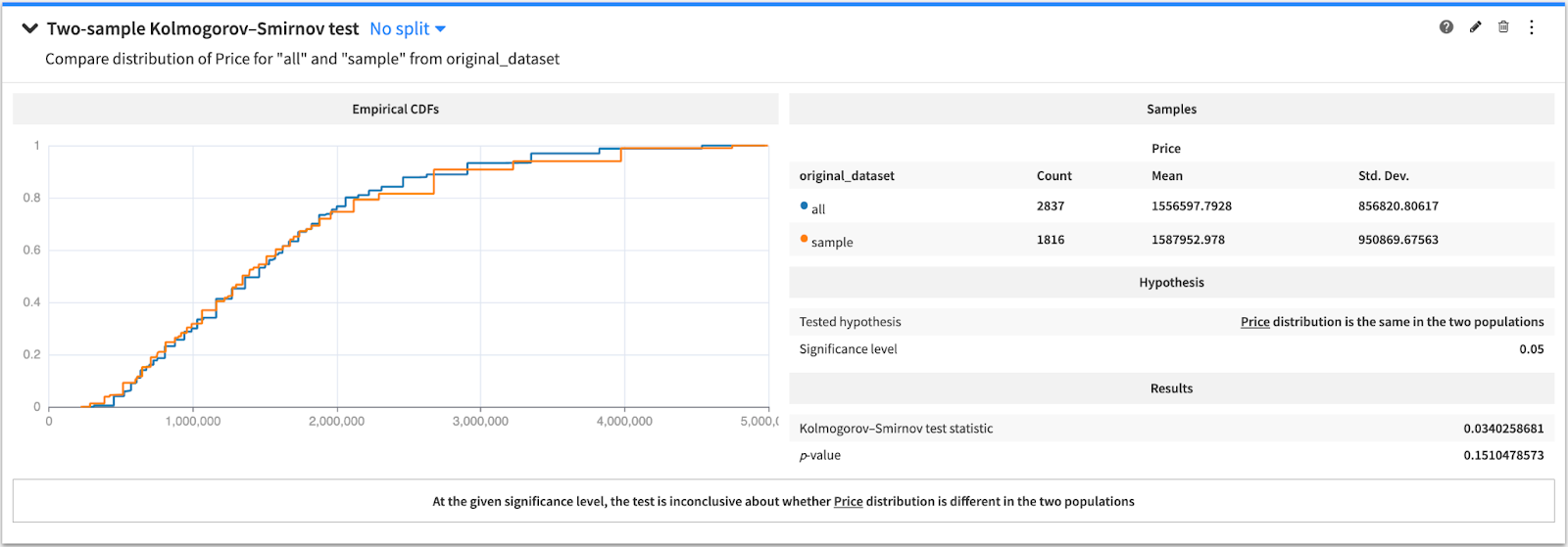
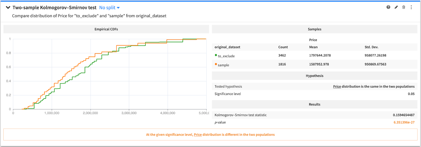
Unfortunately, the dates of the transactions were not collected. However, a large panel of transactions have been exposed by the Dubai land department since 2010 and we will consider those after June 2020 (following the COVID-19 related lockdown). These dated transactions can be used to invalidate (or confirm) the hypothesis that our dataset is representative of the pre-“overpriced” market period (the “pivot” month being June 2021). The two datasets both have the transaction price (but a very few other features in common), and we are going to check that both distributions are similar. 

The proper way to do so is to run the KS statistical test (Kolmogorov-Smirnoff), which can be done from the statistics tab of any dataset within Dataiku. The test will compare the distributions of the two datasets with the null hypothesis (“H0”) being “both samples have a similar distribution.” A significance level of 0.05 is also set.
The test shows that the H0: 

• Is not rejected when using dubai_land data < pivot date
• Is rejected when > pivot date

Hence, we are confident that our dataset is not biased towards the transaction price.

Data Exploration

The statistical observation of the target variable shows us a right skewed distribution, due to extreme “events” (prices) found in the tail of the distribution. Data is indeed not distributed equally on both sides of the distribution’s peak with a long tail found on the right side of the distribution.

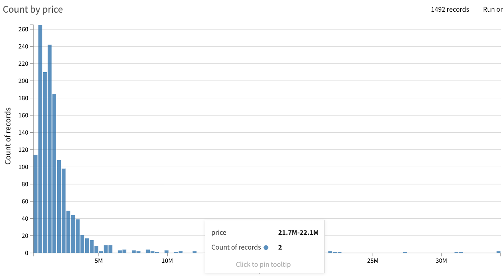
The most extreme observations might even be considered as out of the distribution tail. These samples are commonly different by nature from the others and so ruled by different patterns (in other words, different relationships between variables). As a consequence, they could highly undermine the model performance. A one-dimensional common rule to identify such samples relies on box plots. Box plots are a standardized way of displaying the distribution of data based on statistical measures. 

We label our dataset (“outlier/non-outlier”) according to this rule. Once the target variable has been understood, the dataset can be studied from a two-dimensional perspective through the correlation matrix.

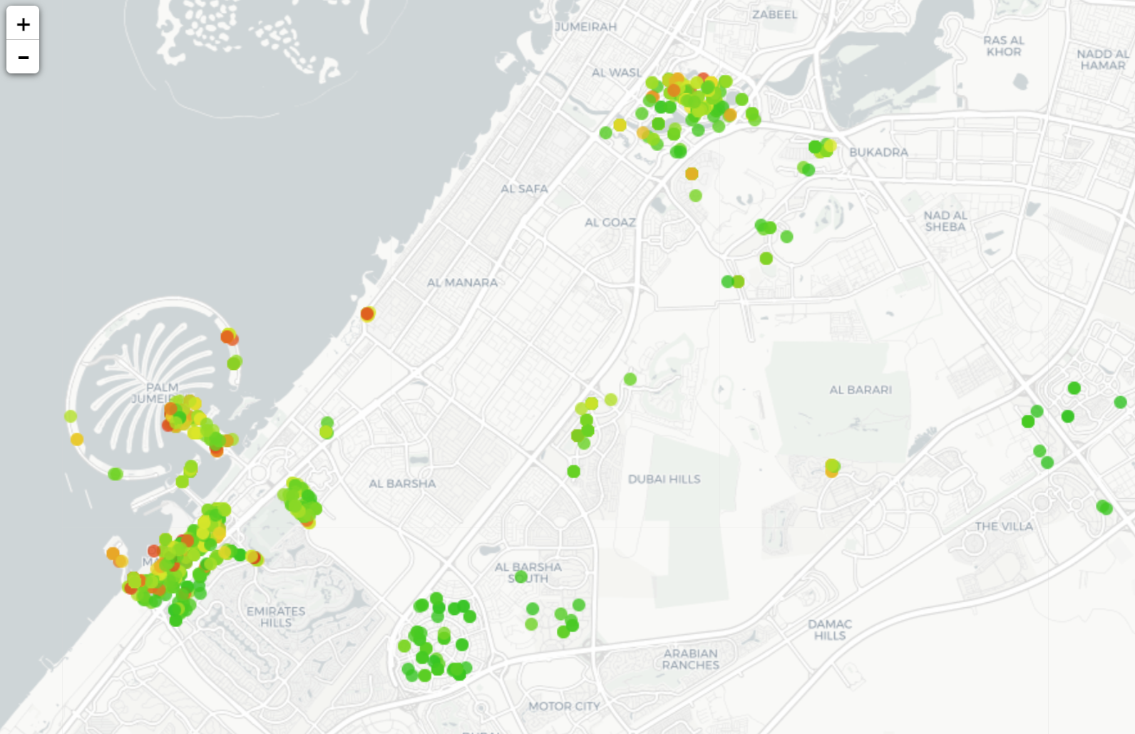
On top of retrieving expected relationships such as a positive correlation between size of apartment, number of rooms, and price, an interesting outcome is the existence of a relationship between the target and the latitude, which is a known behavior: The closer to the seaside, the higher the average price. On the contrary, the price distribution is mainly homogeneous on the longitude line.

Data Preprocessing

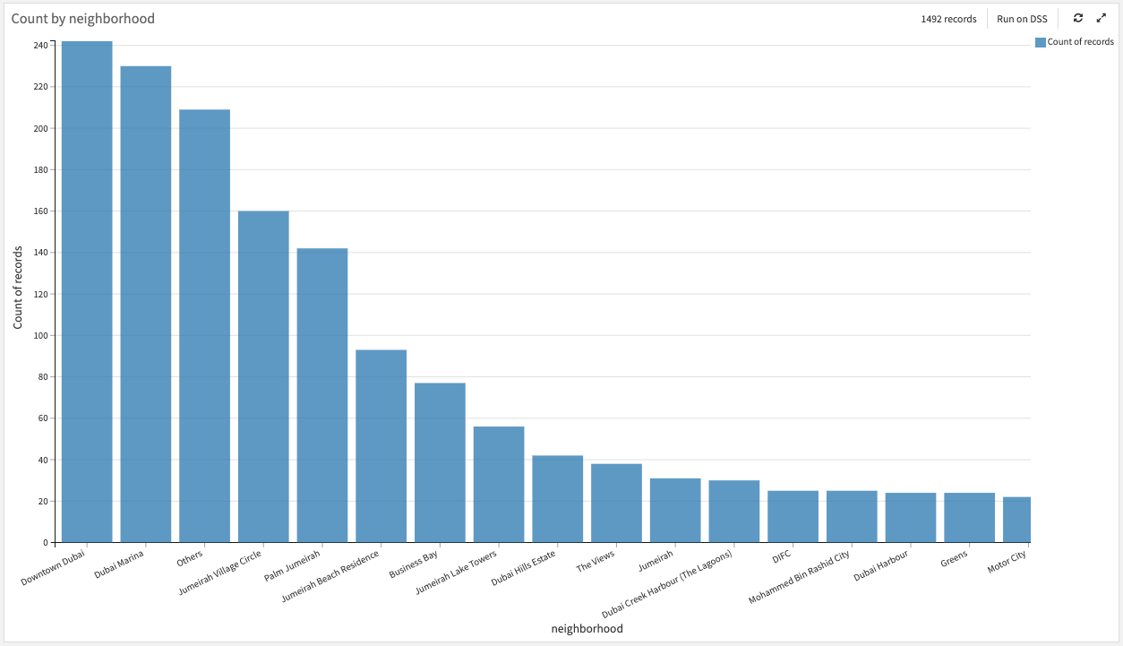
Among the most correlated categorical features with the target, the variable neighborhood  has some modalities observed on very few samples, less than 20. These rare modalities could either have true discriminant information towards the target or lead the model to overfit on them.

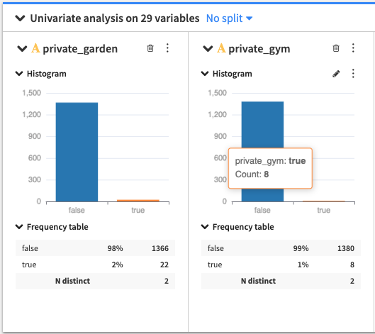
Among these rare modalities, the distribution of the target variable on these most represented does not show that much variance. We choose to group all these rare modalities in a common one that we call “others,” but a more accurate grouping could definitely be done in a further iteration. The same analysis goes for variables with extremely low variance (<0.01) that we remove (private gym / pool / jacuzzi, shared gym, kitchen appliances, etc.). 

Engineering Geo Features

Geo factors affect real estate prices. The geopoints of the properties are known and the location of facilities can be fetched from an API (like maps). And so we derive the proximity to the nearest metro station with the use of a Python recipe and the compute distance processor (of the Prepare visual recipe). That subflow can be made reusable for any other dataset (like the test one) through an app-as-recipe. 

Modeling

The presence of outliers (mentioned earlier) let us anticipate an undermined overall model performance. Indeed, outliers are prone to high magnitude errors, meaning the model will have put more attention on them at the cost of the rest of the dataset. And a quadratic loss such as the MSE (Mean Squared Error) stresses this behavior. (We chose the MSE over gamma regression, as the first is always symmetric and we do not need to weigh one tail more than the other.)

In search of overall model performance and robustness to outliers (and because linear models are sensitive to outliers and so cannot be “trusted,”) the underlying model of the following experiments will be an XGBoost trained with the MSE as loss function and evaluated with the MAPE (Mean Absolute Percentage Error).

We are going to study how to limit the impact of outliers. First, their effect on the model performance has to be measured (through a performance comparison on the test set). Then, based on the performance gain, we will consider “distinguishing” them from the rest of the dataset.

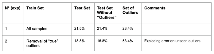
The shift of performance validates their undermining effect on the model. The drawback is the exploding error’s variance on the two sets, which was expected (outliers are not ruled by the same patterns, so the model cannot generalize well on them). 

Clearly, the information of being outlier is highly discriminant for our regression. This variable could actually be used in the decision trees to separate the dataset into outliers / non outliers, and so let the tree learn a specific rule for each of these two populations instead of a common rule when this rule cannot be accurate enough. 

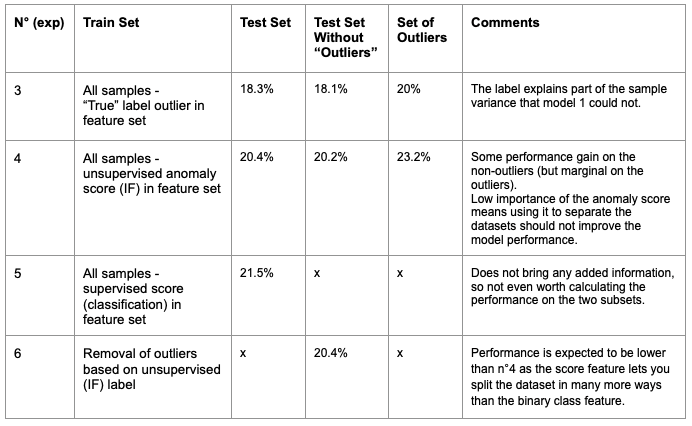
We will create a label outlier variable, based on the true label that we defined earlier. But first, we can have a straightforward estimation of the maximum potential gain brought by such a variable in the model with evaluating the model with the true label as input feature. And such an experiment should return a model with a much more homogeneous distribution of the error and a higher performance.

We tested both supervised and unsupervised techniques for labeling outliers and: 

• Put their output score in the regression model
• Use the output class to separate both train and test sets and evaluate a model specifically on the non-outlier class 

Labeling samples whose true label is based on the (regression) target variable is somehow expected to return limited performance. Still it is interesting to see which of these techniques do best and how important could the gain of performance be.

The logic of the experiments run and their output is shown below. One needs to keep in mind that the set of outliers is of small size and so the “range of confidence” on the computed metrics could be wide:

Our main motivation was to limit the influence (rare) extreme events could have on the majority. In case of separating these two different populations cannot be achieved, uncertainty measures could bring a safer approach. They would indeed consider the entire dataset and return a less certain score on those suspicious points while being robust on the rest of the dataset. One of these techniques is the quantile regression which can return prediction intervals catching the regions of the data with high uncertainty. To conclude, you can explore the fair transaction prices through a webapp (built in Dataiku) exposing the model prediction capability.