In this blog post, we cover some challenges associated with processing and analyzing time series data and how Dataiku features can be used to accelerate modeling such data, along with an example of a project. One of the main challenges comes from the nature of the data, i.e., how it is produced and, thus, how it needs to be processed and structured. We’ll begin with a short discussion of what comprises time series data.
We often use a sequence of time-ordered data points to represent how a measurement changes over time. Such a time series can record events, processes, systems, and so forth. Use cases for time series analysis and prediction include forecasting of quarterly sales, weather, web traffic, and other time-dependent trends.
As a collection of observations (behaviors) for a single subject (entity) at different time intervals, time series data can be collected and analyzed to provide meaningful statistics, charts, and other attributes as general trends and seasonal effects. This data can be used to forecast future values for a time horizon, based on previous observations. Among others, time dependence makes such forecasting challenging. To avoid bias, the model validation technique requires the data to be in chronological order subsequent in time, hence random selection is invalid.
Building good models may be limited by historical data availability and the time domain of records that needs to be finite and equally spaced in frequency. Moreover, underlying patterns in the data as seasonal and trending may drive model performance and the relevant selection process requires data analysis and visualization.
Next, we’ll look at a Dataiku project on time series data by employing preparation and forecasting features available on the platform. The use case predicts the web traffic of Wikipedia articles using historical data. The data is provided in the Kaggle Web Traffic competition. We will discuss our workflow in Dataiku and how we deal with some of these challenges. Readers can further apply the fundamental concepts and tools presented in this article in a wide range of time series projects and subsequently try this or other Kaggle forecasting competitions.
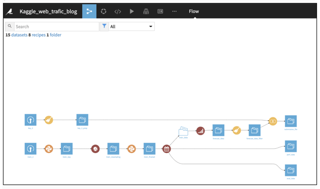
Figure 1: Dataiku Flow
The training dataset consists of approximately 145,000 time series. Each of these time series represent a number of daily views of different Wikipedia articles, starting from July 1, 2015 up until Sept. 1, 2017. The goal of the Kaggle competition was to make predictions of daily views between Sept. 13, 2017 and Nov. 13, 2017 for each article in the dataset. The Dataiku workflow (Figure 1) uses Python recipes and Dataiku plugins. Each plugin contains components that act as a GUI wrapper around some custom code that processes time series data using various Python libraries and machine learning algorithms. The next section walks you through the components for preparing the data and predicting the future web traffic values.
Data Preparation and Analysis
Data cleaning and wrangling are fundamental steps in every data science project and mandatory when working with time series data. A standard format is important so that the programming library used for analysis and forecasting can recognize it as a time series object.
Figure 2: Time Series in Wide Format
We observe our current dataset is in a format of one column corresponding to the web page name feature and multiple to each timestamp. Using Python code, we first transpose the dataset into a standard format of one column representing the Date and, consequently, each distinct time series for the Page is in a separate column known as wide format. The Date is converted into a datetime object and we further reshape the format.
Long format is a compact way of representing multiple time series. In long format as shown in Figure 3, values from distinct time series are stored in the same column called Traffic. The transformed dataset also has an identifier column called Web that provides the web page link for each record. The long format is better at handling irregular and missed visits. Also, the long format has an explicit time variable available that can be used for analysis.
Figure 3: Time Series in Long Format
 Figure 4: Python Script for Dataset Format Transformation
Time series data can occur in irregular time intervals. This creates the need for resampling the frequency of the data. Luckily, the data provided is equispaced and all the time series have the same time interval. However we observe that there are many null values that are filled with zero. A missing value may indicate the traffic was zero or that the data is not available to the day (i.e., the website was created after July 1, 2015).
A widely used technique for inferring missing values for timestamps is the interpolation method, where the missing values do not begin or end the time series. The extrapolation method, on the other hand, is used for prolonging time series that stop earlier than others or start later than others. We use a Dataiku resampling plugin for these time series data transformations.
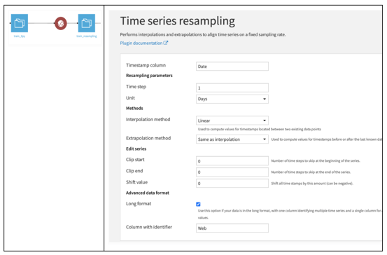 Figure 5: Dataiku Time Series Resampling Plugin
The components of this plugin consist of:
- Time column: This column needs to have parsed dates. In our case, this is the Date column. In the previous sections, we discussed how we parsed columns in the wide format and created Time objects to represent the time series in the long format.
- Time step: This indicates the number of steps between timestamps of the resampled (output) data, specified as a numerical value. We set it to 1 since we want to keep the same frequency of daily records.
- Unit of the Time Step can be specified with a range of choices spanning from Years to Nanoseconds.
- Interpolate / Extrapolate methods are used to fill in empty values as explained earlier.
- Clip / Shift, allow skip and shift of time steps accordingly.
- Long format: As discussed, we’ve created the training dataset in long format, containing multiple time series for various Wikipedia pages, stacked on top of each other. Check Figure 3 again if you need to refresh your memory / cache! If selected, you then have to specify Web as the column that identifies the multiple time series in the Column with identifier parameter.
For each time series, we decided to fill all the records with 0 until the first non-null (i.e., integer) value and then use linear interpolation for any other missing value thereafter. This method fits a line using linear polynomials to construct new points within the range of a discrete set of known data points. Now the data is in the right format to be processed by an algorithm for future values forecasting.
As already mentioned, the model performance may benefit from statistical/exploratory data analysis insights and feature extraction. Exploring this topic in depth is beyond the scope of the post, but a few highlights of the data are outlined here:
1. By taking the sum of traffic for each site during the given period (Figure 6), we observe that the most visited Wikipedia pages in English consist of topics such as Star Wars, Pablo Escobar, and Elizabeth II.
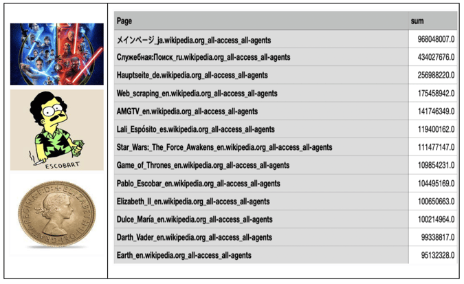 Figure 6: Table Showing the Total Number of Visits for Selected Pages
2. Analyzing specific topics reveal jumps in interest in remarkable events during the time period. For example, by visualizing the SpaceX Falcon 9 page’s traffic in the period of 2015-17, we observe the spike of visits between December 2015 and January 2016. That period marked two successful launches and one successful booster landing.
Figure 7: Web Traffic Visits Over Time for the SpaceX Falcon 9 Page
3. From the string Webpage name, we can extract the language of each page (i.e., de, en, es, fr, ja, ru, zh), the type of access (all, mobile, desktop, spider), and type of agent (spider, non-spider). In other words, each article name has the following format: ‘name_language.wikipedia.org-access_agent' (e.g., 'Millennials_en.wikipedia.org_all-access_all-agents’).
 Figure 8: Python Script for Feature Extraction
4. A sample of the data (Figure 9) shows that English websites have most of the views, while French presents some interesting spikes. Also, Japanese and Spanish show some periodic cycles.
Figure 9: Sample Graph Showing the Web Traffic by Language Over Time
Time Series Modeling
So far, we’ve seen that time series data requires some particular care with regard to the structure of the data. We dealt with it using the Dataiku plugin for data preparation. Time series modeling also requires specific steps to address the nature of the data generation process. These challenges make it a bit different from regular machine learning modeling use cases like classification or regression.
In regression modeling, the goal might be to estimate the value of an unknown target/variable. For example, having analyzed patterns in training data for airline delays, we might attempt to predict the length of the delay for a flight, given a set of features/columns. In time series modeling, the aim is to predict the multiple future values of the same output or measurement.
Second, during the learning process, we need to ensure that the patterns recognized by the algorithms consider the time-dependent nature of the process that leads to the outcomes. As the process we are modeling is time dependent, the ordering of the measurements must be respected. It might be easiest to compare with the approach taken for regression and classification models. In those cases, when we ask the machine to learn patterns in the data, we take random samples as training and test data. For time series modeling, we instead take an ordered sample for our training data and then use the chronologically adjacent data in the set as our test data. We do this sequentially and iteratively to check whether our forecast is right.

Figure 10: Cross Validation Concept
Luckily, the Dataiku forecast plugin can help with most of these steps as well as the actual model training! Let’s have a look at the plugin UI for the options that allow us to do so.
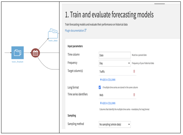 Figure 11: Train and Evaluate Forecasting Models Plugin
The first part of the plugin is used to train forecasting models and evaluate them on historical data. The setting is shown in Figure 11 and the following components are specified:
- Time column: Similar to the resampling recipe, we set the Date as the time component.
- Frequency of the time column: Next, we define the granularity of the time series, from year to minute. This lets the libraries know how to process and learn from the data to create and evaluate models.
- Target column(s): This is the column(s) for which we want to forecast values. We have only one target (univariate forecasting), but we could have multiple columns (multivariate forecasting).
Next, we choose the Forecasting horizon, that is, how many future values of the target column. For the Kaggle submission, we need to forecast two months worth of daily page views of each article. As such, we set the forecasting horizon to over 60 days —65 just to be safe. This way, when we use another recipe in the same plugin, we will get the 65 values for each page, sequentially for that horizon. We’re looking ahead to the final step! Let’s have a short look at the second part of the plugin and the model selection options.
Time Series Forecasting
There are a number of different AutoML choices that let Dataiku make the model selection. In short, the Quick Prototypes use simpler models with preset parameters, whereas the High Performance uses more complex ones. Among others, the AutoML option always picks some standard time series statistical models like the Seasonal naïve method. We used the Expert - Choose Algorithms mode and picked a couple of algorithms to create some initial models. The available choices include statistical models like AutoARIMA and deep learning models such as DeepAR and MQ-CNN from the GluonTS package. The full list of models and parameter defaults is available on the plugin documentation page.
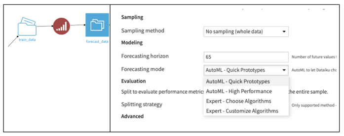 Figure 12: Forecast Future Values Plugin
The final stage consists of evaluation and final output file format. Submissions are evaluated on SMAPE (Symmetric mean absolute percentage error) between forecasts and actual values. We define SMAPE = 0 when the actual and predicted values are both 0. To reduce the submission file size as required by the competition, each page and date combination is given a shorter Id. The mapping between page names and the submission Id can be found in the key files. The final dataset in this project is ready to be uploaded in Kaggle for scoring against real competition values.
The goal of this project was to create a preprocessing and modeling pipeline for time series data on website page views. Using Dataiku features, we processed data on site visits for over 100,000 Wikipedia pages. Thereafter, we dealt with the challenge of structuring the prepared data for applying for training time series models. The Dataiku plugins for resampling, forecasting, and evaluating the models helped with a lot of that work. Also, as and whenever needed, we used Python scripts as code recipes.


