The Nuts and Bolts of Deep Learning Algorithms for Object Detection

You just got a new drone and you want it to be super smart! Maybe it should detect whether workers are properly wearing their helmets or how big the cracks on a factory rooftop are.

In this blog post, we’ll look at the basic methods of object detection (Exhaustive Search, R-CNN, Fast R-CNN and Faster R-CNN) and try to understand the technical details of each model. The best part? We’ll do all of this without any formula, allowing readers with all levels of experience to follow along!

Finally, we will follow this post with a second one, where we will take a deeper dive into Single Shot Detector (SSD) networks and see how this can be deployed… on a drone.

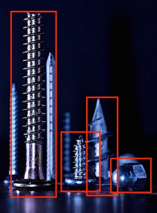Credit: Chris Yates, Unsplash

Our First Steps Into Object Detection

Is It a Bird? Is It a Plane?— Image Classification

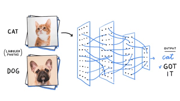Object detection (or recognition) builds on image classification. Image classification is the task of — you guessed it—classifying an image (via a grid of pixels like shown above) into a class category. For a refresher on image classification, we refer the reader to this post.

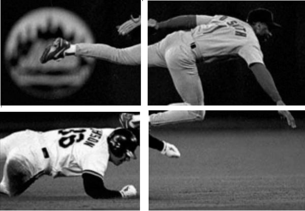
Object recognition is the process of identifying and classifying objects inside an image, which looks something like this:

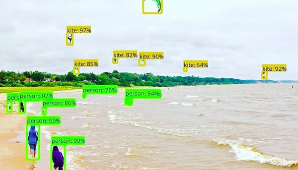
In order for the model to be able to learn the class and the position of the object in the image, the target has to be a five-dimensional label (class, x, y, width, length).

The Inner Workings of Object Detection Methods

A Computationally Expensive Method: Exhaustive Search

The simplest object detection method is using an image classifier on various subparts of the image. Which ones, you might ask? Let’s consider each of them:

1. First, take the image on which you want to perform object detection.

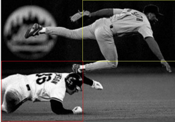
2. Then, divide this image into different sections, or “regions”, as shown below:

3. Consider each region as an individual image.

4. Classify each image using a classic image classifier.

5. Finally, combine all the images with the predicted label for each region where one object has been detected.

One problem with this method is that objects can have different aspect ratios and spatial locations, which can lead to unnecessarily expensive computations of a large number of regions. It presents too big of a bottleneck in terms of computation time to be used for real-life problems.

Region Proposal Methods and Selective Search

A more recent approach is to break down the problem into two tasks: detect the areas of interest first and then perform image classification to determine the category of each object.

The first step usually consists in applying region proposal methods. These methods output bounding boxes that are likely to contain objects of interest. If the object has been properly detected in one of the region proposals, then the classifier should detect it as well. That’s why it’s important for these methods to not only be fast, but also to have a very high recall.

These methods also use a clever architecture where part of the image preprocessing is the same for the object detection and for the classification tasks, making them faster than simply chaining two algorithms. One of the most frequently used region proposal methods is selective search:

Its first step is to apply image segmentation, as shown here:

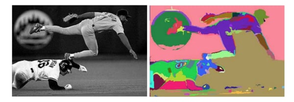
From the image segmentation output, selective search will successively:

1. Create bounding boxes from the segmented parts and add them to the list of region proposals.
2. Combine several small adjacent segments to larger ones based on four types of similarity: color, texture, size, and shape.
3. Go back to step one until the section covers the entire image.
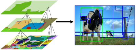   Hierarchical Grouping

Now that we understand how selective search works, let’s introduce some of the most popular object detection algorithms that leverage it.

A First Object Detection Algorithm: R-CNN

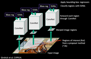
Ross Girshick et al. proposed Region-CNN (R-CNN) which allows the combination of selective search and CNNs. Indeed, for each region proposal (2000 in the paper), one forward propagation generates an output vector through a CNN. This vector will be fed to a one-vs-all classifier (i.e. one classifier per class, for instance one classifier where labels = 1 if the image is a dog and 0 if not, a second one where labels = 1 if the image is a cat and 0 if not, etc), SVM is the classification algorithm used by R-CNN.

But how do you label the region proposals? Of course, if it perfectly matches our ground truth we can label it as 1, and if a given object is not present at all, we can then label it 0 for this object. What if a part of an object is present in the image? Should we label the region as 0 or 1? To make sure we are training our classifier on regions that we can realistically have when predicting an image (and not only perfectly matching regions), we are going to look at the intersection over union (IoU) of the boxes predicted by the selective search and the ground truth:

The IoU is a metric represented by the area of overlap between the predicted and the ground truth boxes divided by their area of union. It rewards successful pixel detection and penalizes false positives in order to prevent algorithms from selecting the whole image.

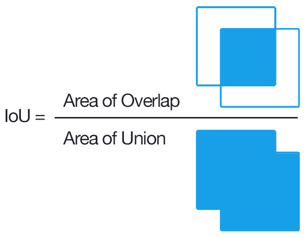
Going back to our R-CNN method, if the IoU is lower than a given threshold (0.3), then the associated label would be 0.

After running the classifier on all region proposals, R-CNN proposes to refine the bounding box (bbox) using a class-specific bbox regressor. The bbox regressor can fine-tune the position of the bounding box boundaries. For example, if the selective search has detected a dog but only selected half of it, the bbox regressor, which is aware that dogs have four legs, will ensure that the whole body is selected.

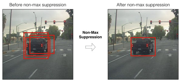
Also thanks to the new bbox regressor prediction, we can discard overlapping proposals using non-maximum suppression (NMS). Here, the idea is to identify and delete overlapping boxes of the same object. NMS sorts the proposals per classification score for each class and computes the IoU of the predicted boxes with the highest probability score with all the other predicted boxes (of the same class). It then discards the proposals if the IoU is higher than a given threshold (e.g., 0.5). This step is then repeated for the next best probabilities.

To sum up, R-CNN follows the following steps:

• Create region proposals from selective search (i.e, predict the parts of the image that are likely to contain an object).
• Run these regions through a pre-trained model and then a SVM to classify the sub-image.
• Run the positive prediction through a bounding box prediction which allows for a better box accuracy.
• Apply an NMS when predicting to get rid of overlapping proposals.

There are, however, some issues with R-CNN:

• This method still needs to classify all the region proposals which can lead to computational bottlenecks — it’s not possible to use it for a real-time use case.
• No learning happens at the selective search stage, which can lead to bad region proposals for certain types of datasets.

A Marginal Improvement: Fast R-CNN

Fast R-CNN — as its name indicates — is faster than R-CNN. It is based on R-CNN with two differences:

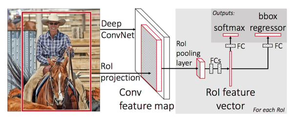
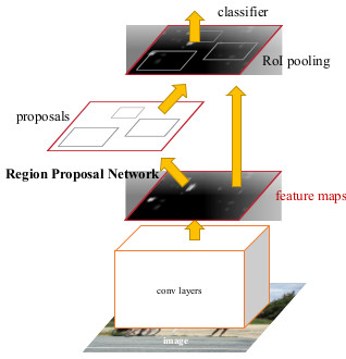
• Instead of feeding the CNN for every region proposal, you feed the CNN only once by taking the whole image to generate a convolutional feature map (take a vector of pixels and transform it into another vector using a filter which will give you a convolutional feature map — you can find more info here). Next, the region of proposals are identified with selective search and then they are reshaped into a fixed size using a Region of Interest pooling (RoI pooling) layer to be able to use as an input of the fully connected layer.
• Fast-RCNN uses the softmax layer instead of SVM in its classification of region proposals which is faster and generates a better accuracy.

Here is the architecture of the network:

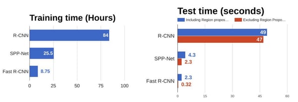
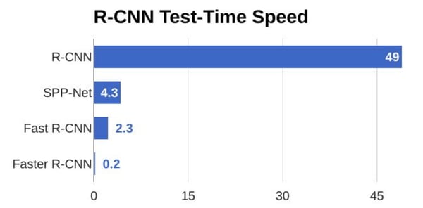
As we can see in the figure below, Fast R-CNN is way faster at training and testing than R-CNN. However, a bottleneck still remains due to the selective search method.

How Fast Can R-CNN Get? — FASTER R-CNN

While Fast R-CNN was a lot faster than R-CNN, the bottleneck remains with selective search as it is very time consuming. Therefore, Shaoqing Ren et al. came up with Faster R-CNN to solve this and proposed to replace selective search by a very small convolutional network called Region Proposal Network (RPN) to find the regions of interest.

In a nutshell, RPN is a small network that directly finds region proposals.

One naive approach to this would be to create a deep learning model which outputs x_min, y_min, x_max, and x_max to get the bounding box for one region proposal (so 8,000 outputs if we want 2,000 regions). However, there are two fundamental problems:

• The images can have very different sizes and ratios, so to create a model correctly predicting raw coordinates can be tricky.
• There are some coordinate ordering constraints in our prediction (x_min < x_max, y_min < y_max).

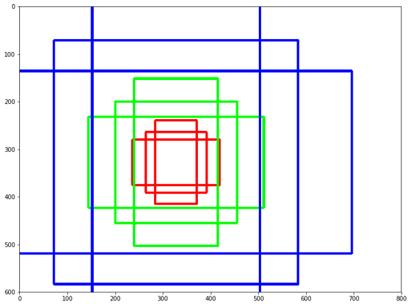
To overcome this, we are going to use anchors:

Anchors are predefined boxes of different ratios and scales all over the image. For example, for a given central point, we usually start with three sets of sizes (e.g., 64px, 128px, 256px) and three different width/height ratios (1/1, ½, 2/1). In this example, we would end up having nine different boxes for a given pixel of the image (the center of our boxes).

So how many anchors would I have in total for one image?

It is paramount to understand that we are not going to create anchors on the raw images, but on the output feature maps on the last convolutional layer. For instance, it’s false to say that for a 1,000*600 input image we would have one anchor per pixel so 1,000*600*9 = 5,400,000 anchors. Indeed, since we are going to create them on the feature map, there is a subsampling ratio to take into account (which is the factor reduction between the input and the output dimension due to strides in our convolutional layer).

In our example, if we take this ratio to be 16 (like in VGG16) we would have nine anchors per spatial position of the feature map so “only” around 20,000 anchors (5,400,000 / 16²). This means that two consecutive pixels in the output features correspond to two points which are 16 pixels apart in the input image. Note that this down sampling ratio is a tunable parameter of Faster R-CNN.

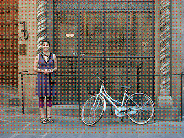Center of the anchors

The remaining question now is how to go from those 20,000 anchors to 2,000 region proposals (taking the same number of region proposals as before), which is the goal of our RPN.

How to Train the Region Proposal Network

To achieve this, we want our RPN to tell us whether a box contains an object or is a background, as well as the accurate coordinates of the object. The output predictions are probability of being background, probability of being foreground, and the deltas Dx, Dy, Dw, Dh which are the difference between the anchor and the final proposal).

• First, we will remove the cross-boundary anchors (i.e. the anchors which are cut due to the border of the image) — this left us with around 6,000 images.
• We need to label our anchors positive if either of the two following conditions exist:

→ The anchor has the highest IoU with a ground truth box among all the other anchors.

→ The anchor has at least 0.7 of IoU with a ground truth box.

• We need to label our anchors negative if its IoU is less than 0.3 with all ground truth boxes.
• We disregard all the remaining anchors.
• We train the binary classification and the bounding box regression adjustment.

Finally, a few remarks about the implementation:

1. We want the number of positive and negative anchors to be balanced in our mini batch.
2. We use a multi-task loss, which makes sense since we want to minimize either loss — the error of mistakenly predicting foreground or background and also the error of accuracy in our box.
3. We initialize the convolutional layer using weights from a pre-trained model.

How to Use the Region Proposal Network

• All the anchors (20,000) are scored so we get new bounding boxes and the probability of being a foreground (i.e., being an object) for all of them.
• Use non-maximum suppression (see the R-CNN section)
• Proposal selection: Finally, only the top N proposals sorted by score (with N=2,000, we are back to our 2,000 region proposals) are kept.

We finally have our 2,000 proposals like in the previous methods. Despite appearing more complex, this prediction step is way faster and more accurate than the previous methods.

The next step is to create a similar model as in Fast R-CNN (i.e. RoI pooling, and a classifier + bbox regressor), using RPN instead of selective search. However, we don’t want to do exactly as before, i.e. take the 2,000 proposals, crop them, and pass them through a pre-trained base network. Instead, reuse the existing convolutional feature map. Indeed, one of the advantages of using an RPN as a proposal generator is to share the weights and CNN between the RPN and the main detector network.

1. The RPN is trained using a pre-trained network and then fine-tuned.
2. The detector network is trained using a pre-trained network and then fine-tuned. Proposal regions from the RPN are used.
3. The RPN is initialized using the weights from the second model and then fine-tuned—this is going to be our final RPN model).
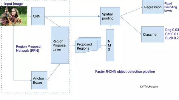
4. Finally, the detector network is fine-tuned (RPN weights are fixed). The CNN feature maps are going to be shared amongst the two networks (see next figure).
   Faster R-CNN network

To sum up, Faster R-CNN is more accurate than the previous methods and is about 10 times faster than Fast-R-CNN, which is a big improvement and a start for real-time scoring.

Even still, region proposal detection models won’t be enough for an embedded system since these models are heavy and not fast enough for most real-time scoring cases — the last example is about five images per second.

In our next post, we will discuss faster methods like SSD and real use cases with image detection from drones. We’re excited to be working on this topic for Dataiku DSS — check out the additional resources below to learn more:

• Object detection plugin for Dataiku DSS projects
• This NATO challenge we won at Dataiku using an object detection algorithm