


In the last post in the Top Machine Learning Algorithms: How They Work (In Plain English!) series, we went through a basic overview of machine learning and introduced a few key categories of algorithms and explored the most basic one, linear models. Now, let’s dive into the next category, tree-based models.
Tree-based models use a series of if-then rules to generate predictions from one or more decision trees. All tree-based models can be used for either regression (predicting numerical values) or classification (predicting categorical values). We’ll explore three types of tree-based models:
- Decision tree models, which are the foundation of all tree-based models.
- Random forest models, an “ensemble” method which builds many decision trees in parallel.
- Gradient boosting models, an “ensemble” method which builds many decision trees sequentially.

Tree-Based Models in Action: Practical Examples
If you missed the first post in this series, see here for some background on our use case. TL;DR let’s pretend we’re the owners of Willy Wonka’s Candy Store, and we want to better predict customer spend. We’ll explore a specific customer, George — a 65-year-old mechanic with children who spent $10 at our store last week — and predict whether he will be a “high spender” this week.
Decision Tree Models
First, let’s start with a simple decision tree model. A decision tree model can be used to visually represent the “decisions”, or if-then rules, that are used to generate predictions. Here is an example of a very basic decision tree model:
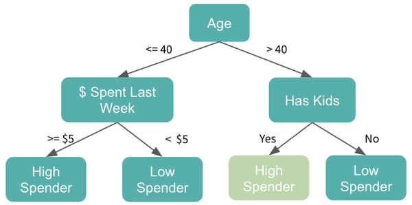
We’ll go through each yes or no question, or decision node, in the tree and will move down the tree accordingly, until we reach our final predictions. Our first question, which is referred to as our root node, is whether George is above 40 and, since he is, we will then proceed onto the “Has Kids” node. Because the answer is yes, we’ll predict that he will be a high spender at Willy Wonka Candy this week.
One other note to add — here, we’re trying to predict whether George will be a high spender, so this is an example of a classification tree, but we could easily convert this into a regression tree by predicting George’s actual dollar spend. The process would remain the same, but the final nodes would be numerical predictions rather than categorical ones.
How Do We Actually Create These Decision Tree Models?
Glad you asked. There are essentially two key components to building a decision tree model: determining which features to split on and then deciding when to stop splitting.
When determining which features to split on, the goal is to select the feature that will produce the most homogenous resulting datasets. The simplest and most commonly used method of doing this is by minimizing entropy, a measure of the randomness within a dataset, and maximizing information gain, the reduction in entropy that results from splitting on a given feature.
We’ll split on the feature that results in the highest information gain, and then recompute entropy and information gain for the resulting output datasets. In the Willy Wonka example, we may have first split on age because the greater than 40 and less than (or equal to) 40 datasets were each relatively homogenous. Homogeneity in this sense refers to the diversity of classes, so one dataset was filled with primarily low spenders and the other with primarily high spenders.
You may be wondering how we decided to use a threshold of 40 for age. That’s a good question! For numerical features, we first sort the feature values in ascending order, and then test each value as the threshold point and calculate the information gain of that split.
The value with the highest information gain — in this case, age 40 — will then be compared with other potential splits, and whichever has the highest information gain will be used at that node. A tree can split on any numerical feature multiple times at different value thresholds, which enables decision tree models to handle non-linear relationships quite well.
The second decision we need to make is when to stop splitting the tree. We can split until each final node has very few data points, but that will likely result in overfitting, or building a model that is too specific to the dataset it was trained on. This is problematic because, while it may make good predictions for that one dataset, it may not generalize well to new data, which is really our larger goal.
To combat this, we can remove sections that have little predictive power, a technique referred to as pruning. Some of the most common pruning methods include setting a maximum tree depth or minimum number of samples per leaf, or final node.
Here’s a high-level recap of decision tree models:
Advantages:- Straightforward interpretation
- Good at handling complex, non-linear relationships
- Predictions tend to be weak, as singular decision tree models are prone to overfitting
- Unstable, as a slight change in the input dataset can greatly impact the final results
Ensemble Methods
While pruning is a good method of improving the predictive performance of a decision tree model, a single decision tree model will not generally produce strong predictions alone. To improve our model’s predictive power, we can build many trees and combine the predictions, which is called ensembling. Ensembling actually refers to any combination of models, but is most frequently used to refer to tree-based models.
The idea is for many weak guesses to come together to generate one strong guess. You can think of ensembling as asking the audience on “Who Wants to Be a Millionaire?” If the question is really hard, the contestant might prefer to aggregate many guesses, rather than go with their own guess alone.

To get deeper into that metaphor, one decision tree model would be the contestant. One individual tree might not be a great predictor, but if we build many trees and combine all predictions, we get a pretty good model! Two of the most popular ensemble algorithms are random forest and gradient boosting, which are quite powerful and commonly used for advanced machine learning applications.
Bagging and Random Forest Models
Before we discuss the random forest model, let’s take a quick step back and discuss its foundation, bootstrap aggregating, or bagging. Bagging is a technique of building many decision tree models at a time by randomly sampling with replacement, or bootstrapping, from the original dataset. This ensures variety in the trees, which helps to reduce the amount of overfitting.
Random forest models take this concept one step further. On top of building many trees from sampled datasets, each node is only allowed to split on a random selection of the model’s features.
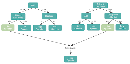
For example, imagine that each node can split from a different, random selection of three features from our feature set. Looking at the above, you may notice that the two trees start with different features — the first starts with age and the second starts with dollars spent. That’s because even though age may be the most significant feature in the dataset, it wasn’t selected in the group of three features for the second tree, so that model had to use the next most significant feature, dollars spent, to start.
Each subsequent node will also split on a random selection of three features. Let’s say that the next group of features in the “less than $1 spent last week” dataset included age, and this time, the age 30 threshold resulted in the highest information gain among all features, age greater or less than 30 would be the next split.
We’ll build our two trees separately and get the majority vote. Note that if it were a regression problem, we would get the average.
Here’s a high-level recap of random forests:
Advantages:- Good at handling complex, non-linear relationships
- Handle datasets with high dimensionality (many features) well
- Handle missing data well
- They are powerful and accurate
- They can be trained quickly. Since trees do not rely on one another, they can be trained in parallel.
Disadvantages:
- Less accurate for regression problems as they tend to overfit
Boosting and Gradient Boosting
Boosting is an ensemble tree method that builds consecutive small trees — often only one node — with each tree focused on correcting the net error from the previous tree. So, we’ll split our first tree on the most predictive feature and then we’ll update weights to ensure that the subsequent tree splits on whichever feature allows it to correctly classify the data points that were misclassified in the initial tree. The next tree will then focus on correctly classifying errors from that tree, and so on. The final prediction is a weighted sum of all individual predictions.
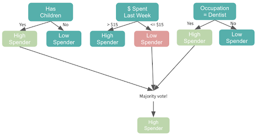
Gradient boosting is the most popular extension of boosting, and uses the gradient descent algorithm for optimization.
Here’s a high-level recap of gradient boosting:
Advantages:- They are powerful and accurate, in many cases even more so than random forest
- Good at handling complex, non-linear relationships
- They are good at dealing with imbalanced data
Disadvantages:
- Slower to train, since trees must be built sequentially
- Prone to overfitting if the data is noisy
- Harder to tune hyperparameters
Recap
Tree-based models are very popular in machine learning. The decision tree model, the foundation of tree-based models, is quite straightforward to interpret, but generally a weak predictor. Ensemble models can be used to generate stronger predictions from many trees, with random forest and gradient boosting as two of the most popular. All tree-based models can be used for regression or classification and can handle non-linear relationships quite well.
We hope that you find this high-level overview of tree-based models helpful and be sure to stay on the lookout for future posts from this series discussing other families of algorithms.