


Full disclaimer: I am a bit of a data science beer geek. A few years ago, I scraped a beer rating website, and at the time, I wanted to test different recommendation algorithms. More recently, I was advised to follow this excellent class by Charles Ollion (Heuritech) and Olivier Grisel to learn more about some specific aspects of deep learning. When I came across the second lab on factorization machine and deep recommendations, I remembered my old beer dataset and decided to give it a shot.
In the following blog post, I’ll discuss the different experiments I was able to run using Keras. I did the project using Python, pandas, scikit-learn and Keras. Throughout the blog post, I’ll share the Keras code when it seems appropriate. To make it easier to follow, you can also check out the complete Ipython notebook.
The Data
Ratings
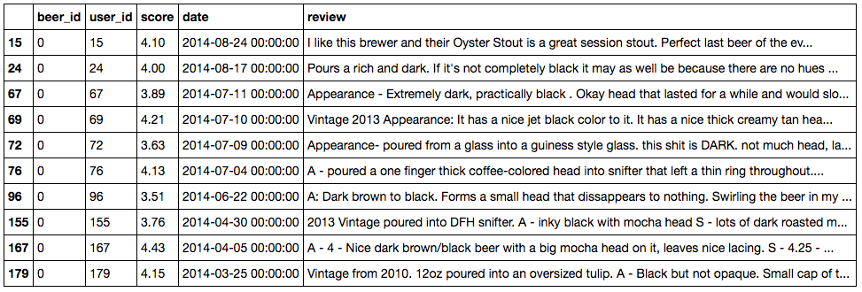
We scraped a beer rating website and ended up with several datasets. The most important one contains the reviews (scores given by the users) and is composed of:
- “beer_id”: a unique id for a beer
- “user_id”: a unique id for a user
- “score”: the review score, between 1 and 5
- “date”: the timestamp of when the user posted the review
- “review”: a review of the beer. This is optional, and left empty 75 % of the time. I won’t use this information in this blog post though it would be interesting to integrate it somehow.
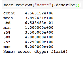
In total, I got 4.563.152 ratings. Here is a head of this dataset:
You can notice that most scores seem to be between 3.75 and 4.25. We can get an idea of the ratings distribution using pandas:
And by plotting the distribution:
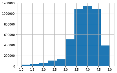
The median is 4. This is very important because it means the ratings are skewed toward high values. This is a common bias in internet ratings where people tend to rate items or movies that they liked and rarely spend time to comment something they dislike or are indifferent to (unless they are haters, of course). This distribution shape will have a big impact on the results of our recommendation engines — I’ll discuss this further later on.
In the review dataset, we have 91,645 distinct users and 78,518 beers. This means that on average, each user has rated around 50 beers, which seems quite high. So I looked for answers to the questions: How many ratings do we have per beer? Per user? What are the corresponding distributions?
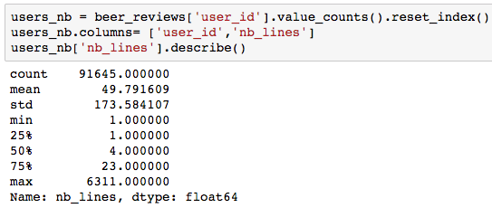
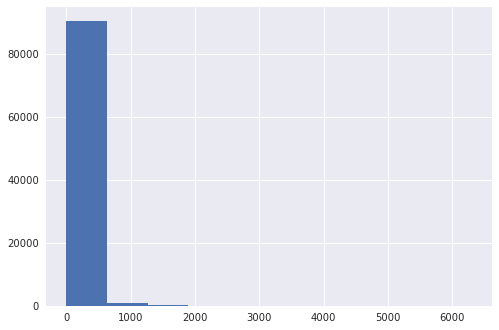
As expected, the distribution is very skewed, with 50% of people having done no more than four reviews (and one person going crazy with more than 6,000 ratings...or is it a bot?)! This has the following implications: we will have few beers to characterize most users, but for at least 25% of the users, we will have at least 23 ratings. This is probably enough information to start generating good recommendations.
Now let’s have a look at the beers:
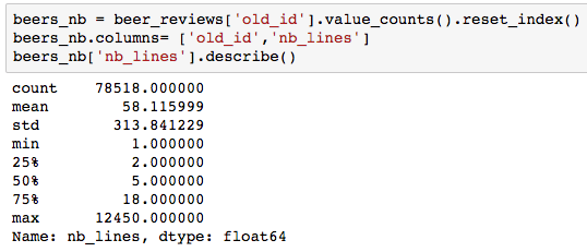
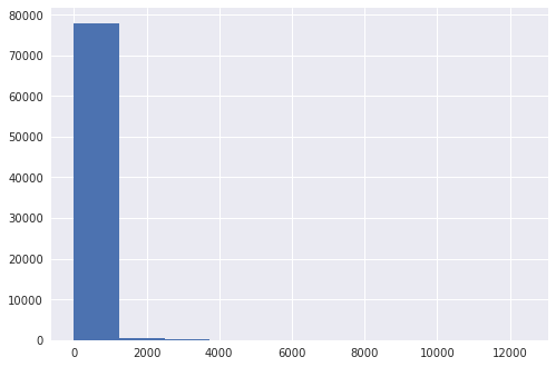
Again, the distribution is very skewed, with 50% of the beers having five ratings or less. Even worse, 75% of beers have less than 18 ratings. Though this distribution is expected for users, I assumed the distribution of beer counts to be less skewed, with a good number of well-known beers.
Metadata
I scraped information about each beer as well: the brewery with which they are associated as well as user data. With this, I can extend the analysis by adding some “beer geek knowledge.” Let’s have a look at the beers that received the most ratings, for example.
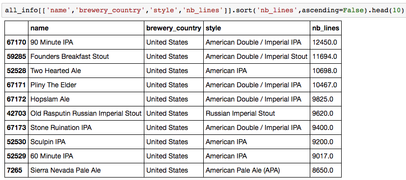
Though I know most of these beers, some of them do not ring a bell at all. This is because of two biases:
- Most of the users probably come from the United States, which explains why all of the most rated beers above are from there. I am on the other side, from France. In France, we can find some of these beers (like the Sierra, Stone or Founder). However, only in dedicated shops. Thus, the beers are more likely purchased by a specific population, which leads us to the second bias.
- Most of the people rating beers on this website have a “beer geek” profile. Since they will rate mostly beers they liked, we can expect the most rated beer to be US common-quality craft beers. To me, that’s 90 Minute IPA or Sierra Nevada.
We can verify the first assumption by looking at the user metadata:
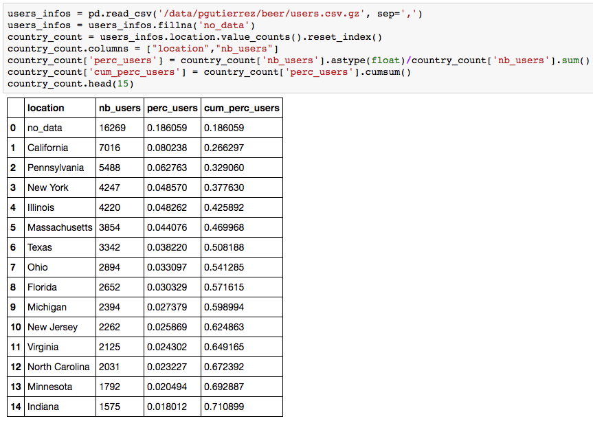
So we have around 20% of unknown locations and more than 50% American users. In fact if we look at the non-US entries in the list, we get:
- The state of Ontario(Canada) as the first entry, with 718 users.
- United Kingdom and Australia as the two first countries, with 348 and 306 users, respectively.
- France arrives at the 69th position with 62 users. Sad.
These metadata enable us to understand biases that appear in the model, but they can also be used in the recommendation system (see Part 3). Finally, let’s have a look at the bottom- and top-rated beers.
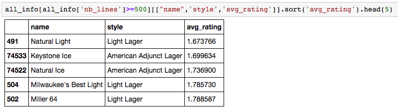
I have to say is that I have never tried any of these beers. You can’t really find light beers in France, but this seems to confirm both biases. All beers come from the United States, and light beers will be rated low here because they do not target a beer geek audience. Let’s take a look at the top ones:
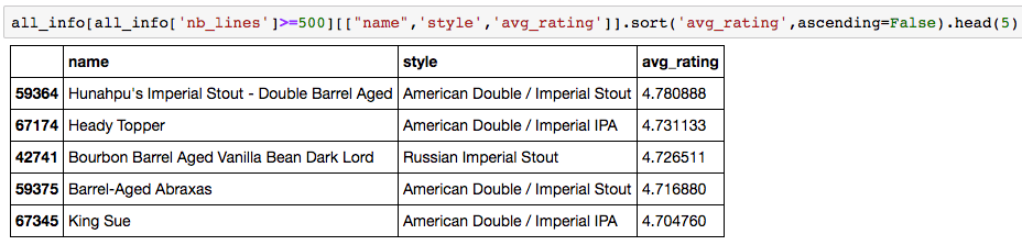
I have no idea what these beers are. This may be because the best beers (according to our ratings) are probably craft beers and hence less well-spread. However, we see that the best-rated beers are all imperial (Stout or IPA), which is — again — expected.
Our First Explicit Recommendation Engine
Explicit or Implicit recsys
You can learn more about the different types of neural recommender systems as well as explicit vs implicit recommendation engines in the excellent slides by Ollion and Grisel.
Basically, explicit feedback is when your users voluntarily give you information on what they like and dislike. In our case, we have explicit beer ratings ranging from one to five. Other examples would be the reviews you can see on Amazon (see their dataset) or on MovieLens (a well known dataset for recommendation engines).
However, in many cases, we don’t have this information or it is not rich enough. Thus, we need to extract implicit information from the interaction between the system and the user. For example, when you type a Google query, you do not explicitly notify Google of the search result pertinence. But you do click on one or more of the proposed links and spend a certain amount of time on the corresponding pages. That’s implicit feedback that Google can take into account to increase its search engine performance. Following the same idea, most people won’t rate their purchase on Amazon, giving no explicit feedback. However, Amazon can record all products searched, viewed, or purchased to infer customer tastes.
Back to our beer recommendation engine. The implicit information could be anything, like the website pages visited, time spent on these pages, etc. However, in the data, I only have ratings. The implicit information can also simply be the list of beers people reviewed (or drank), i.e., for all possible tuple (user,item) 1 for beer drank, else 0. Though this information seems less rich than a rating, it helps the system understand what people do not drink and might dislike.
In what follows, I will start with the explicit recommendation engine. It basically boils down to a regression problem where I try to predict the ratings for each user. This means that I will recommend a beer to a user that (s)he is likely to rate highly upon drinking.
To evaluate the model, I randomly split the data into training and test sets. Note that I could do things more properly by splitting the user ratings based on increasing timestamps — this would make it possible to predict the next beers a user will drink. But I’ll leave this aside for now.
Matrix Factorization
Now that I’ve described the data and the method, let’s create a simple model using Keras. For the algorithm in Keras to work, I had to remap all beers and user ids to an integer between 0 and either the total number of users or the total number of beers.
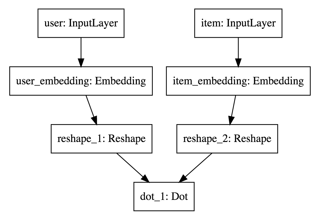
My first model will be based on a matrix factorization approach. The idea is to project beers and users in a common latent space. In Keras, we can define our model this way:
What I’m doing is creating an embedding for the users and one for the items. The dot product between an item and a product is the rating prediction. When I train the model, the embeddings parameters are learned, which gives me a latent representation.
In the code:
- Line 1 and 2 we declare inputs to the model.
- Line 4 we define the size of embeddings as a parameter.
- Line 5 to 8 we apply an embedding layer to both beer and user inputs.
- Line 10 and 11 reshape from shape (batch_size, input_length,embedding_size) to (batch_size, embedding_size). A Flatten layer can be used as well.
- Line 13 declare our output as being the dot product between the two embeddings.
- We declare a model (Line 15) that takes beers and users as input and output y, our prediction.
- This model need to be compiled with the right loss and optimizer (line 17).
Notice that Keras provide a way to display each model as svg or save them as images.
Which gives us, the very readable
To train the model, we simply need to call the model’s fit method (because our dataset fits in memory, else we could have used fit_generator).
The code from lines 1 to 8 and 17 to 19 allows me to save histories and best models (with Keras callbacks). Notice also that I use an internal random cross validation scheme (the validation_split=0.1 parameter). This is because I’m going to grid search several parameters and architectures. Since I’m exploring and going to follow the most promising leads, I will be prone to manually overfit. The test set will be kept to verify the quality of recommendations at the end of part 3.
Here’s what I get when I plot the training and evaluation MSE loss:
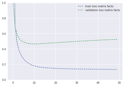
The training loss stabilizes around 0.15. After 10 epochs, the model starts overfitting — the best MSE validation loss is around 0.465. A quick grid search on the embedding sizes gives me:
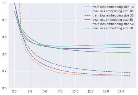
This shows that choosing large values of embedding sizes leads to overfitting. Hence, for most of the experimentations I’ll keep this embedding size of 10 (giving me around 0.42 validation mse). Now, let’s go deeper.
Going Deeper
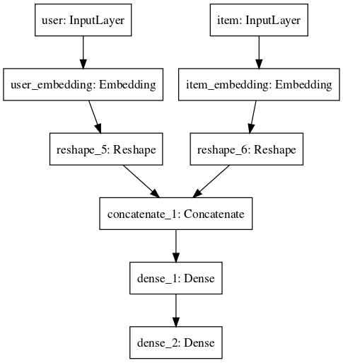
Using the architecture above, I’m trying to predict a rating by performing a dot product. The dot product enables the model to perform the matrix factorization approach. But we can relax this dot structure by instead using whatever network we want to predict the rating. For example, I can use a concatenate layer followed by a dense layer. This means that instead of relying on a simple dot product, the network can find the way it wants to combine the information itself.
With a two layer deep neural network, this gives us using Keras:
This is exactly the same code as before, except I changed the Dot layer by a Concatenate layer followed by several Dense ones. Here is the model representation that can be compared to the previous one:
When training the model, I get the following chart:
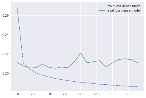
It’s worth noting that though my training error goes down with a rather common shape, the validation error plateaus after just one or two iterations. But did I get better? Here’s a graph of the comparison with the previous best model:
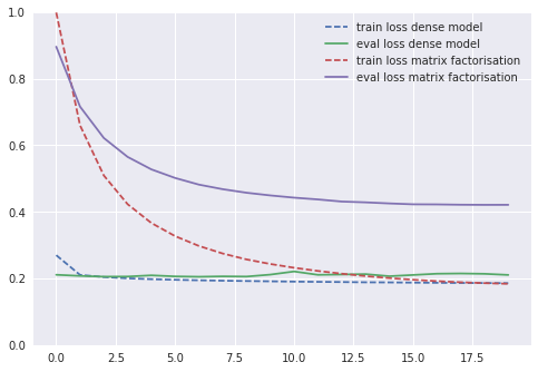
Obviously, the performance got way better! From 0.42 to 0.20 validation loss. We can also notice the following points:
- We converge really fast to the best model. After one or two epochs, the model starts overfitting or at least the validation loss does not seem to go down anymore.
- When comparing to the previous model, we almost manage to match the training error with our validation error! This may mean that we are close to reaching the best possible validation error.
- I actually added some dropout in this architecture. It gives me a few extra points.
I can also grid search around this architecture. What happens if I add another layer on top of the first one? What happens if I decrease the embedding size? (Modifications commented in the code above.)
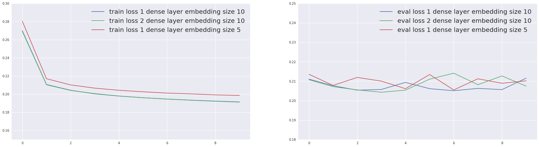
Adding a layer does not help much. The training error is quite similar, even if I may get a little improvement on the validation loss. In the opposite direction, simplifying the model by reducing embedding size worsens the training and validation errors. That’s it! I showed how to create our first matrix factorization and deep models.