


Recently, Graph Neural Networks (GNNs) have received a lot of attention. From marketing to social science to biology, they have been widely promoted as the new way of learning “smartly” from data. It’s more than a trend, though, as many research papers have proven that they can actually lead to more accurate and robust models.
What could possibly explain this? This is certainly due to their ability to combine graphical representation learning (which is used today for a wider variety of use cases) with the predictive power of deep learning models.
Objective
This article is the first part of three-part series that aims to provide a comprehensive overview of the most common applications of GNN models to real-world problems.
While the first focuses on node classification, the two others tackle link prediction and graph classification, respectively.
After reading this article, you will understand:
- What is graphical representation learning all about?
- What are the main mechanisms hidden under GNNs models?
- How can they be applied to real-world classification problems?
The experimentations described in the article were carried out using the libraries PyTorch Geometric, NetworkX, igraph, and Plotly. You can find the code here on GitHub.
1. Graphical Representation Learning: What Is It All About?
1.1 Motivation
The first question you are likely to ask yourself is why and when should you consider graphical representation learning to solve your use case?
Graphs provide a simple yet powerful tool to describe complex systems. In simple terms, it consists of representing a problem as a set of objects (nodes) along with a set of interactions (edges) between pairs of these objects.
Yet, the number of applications where data is represented in the form of graphs is important. Here are some examples:
- Recommender Systems: In e-commerce, you can represent interactions between users and products graphically and use this knowledge to make more relevant personalized recommendations.
- Social Networks: By using a graph to describe the relationship between users, you can train a model to detect fake accounts.
- Transport: Networks can be visualized as a graph and used as inputs by models to accurately forecast traffic speed, volume, or density.
- Chemistry: Molecules are usually modeled as graphs. By using this representation, you can predict their bioactivity for drug discovery purposes.
1.2 Benefits
The second question you might consider is: What do graph-based models bring to the table compared to “traditional” approaches?The key advantage of using a graphical representation of a problem lies in its ability to represent both information about the points and relationships between nodes.
To put it more concretely, let’s consider the case where you would like to classify products sold in a store. You would probably gather information about the products (description, price, brand, etc.) and use it as input to train a model. But what if this information is non-existent or too poor to build a robust model?
In this context, you can leverage the graphical aspect of the problem. Each product can be represented as a node and each pair of products frequently bought together can be linked. A graph-based model is then likely to perform better than a “traditional” machine learning algorithm, as it would learn not only from information about products but also from the relationships between them. In fact, instead of considering each product independently, it would leverage this additional information to detect valuable patterns.
1.3 Prediction Tasks on Graphs
Before going further, it is important to distinguish between three main types of tasks for which graph-based models can be used for:
Node-level tasks: Node classification and regression
- Goal: Predict a label, type, category, or attribute of a node.
- Example: Given a large social network with millions of users, detect fake accounts.
Edge-level tasks: Link prediction
- Goal: Given a set of nodes and an incomplete set of edges between these nodes, infer the missing edges.
- Example: Predict biological interactions between proteins.
Graph-level tasks: Graph classification, regression, and clustering
- Goal: Carry a classification, regression, or clustering task over entire graphs.
- Example: Given a graph representing the structure of a molecule, predict molecules’ toxicity.
In the rest of the article, I will focus on node classification.
2. Node Classification With GNN: What Performance Should You Expect?
2.1 Description of the Use Case
Imagine that you run a large online knowledge-sharing platform such as Wikipedia. Every day, thousands of scientific articles are published.
To help your readers easily navigate the platform and find the content they are interested in, you need to make sure that each article is classified into the right category quickly after its publication.
In this context, the problem can be modeled as a graph where each node represents an article and has as an attribute an embedding of the content. Two articles are linked if one of them contains a link to the other. The goal is to predict the category of new articles.
This is thus a typical node classification task!
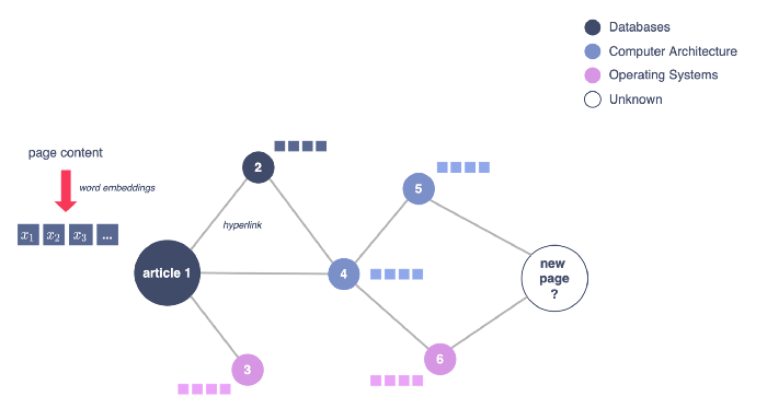
Figure 1 - Graphical representation of the use case, illustration by Lina Faik
The dataset I will be using for experiments is Wiki-CS from the paper Wiki-CS: A Wikipedia-Based Benchmark for Graph Neural Networks. It consists of nodes corresponding to computer science articles, with edges based on hyperlinks and 10 classes that represent different branches of the field. You can download it using PyTorch datasets here.
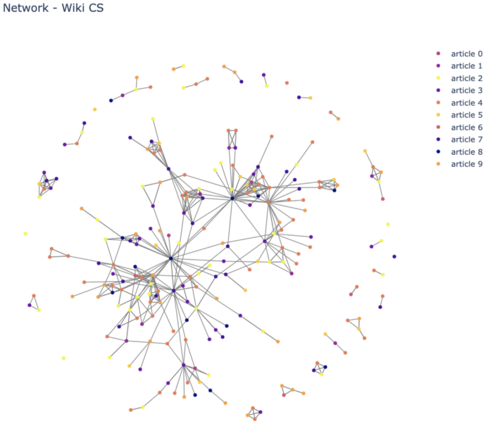
Figure 2 - Projection of a subset of the graph, illustration by Lina Faik
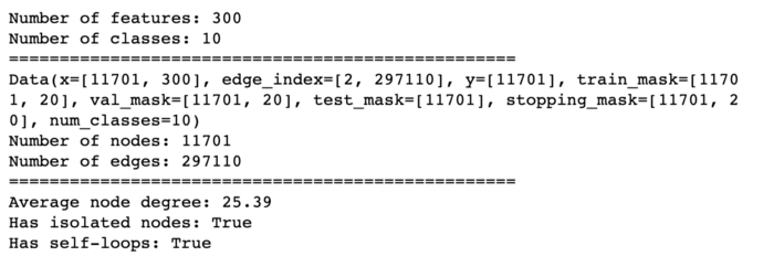
Figure 3 - Basic information and statistics about the graph, illustration by Lina faik
Challenges
The nature of graph data poses a real challenge to existing deep learning models. Why?
- Non-Euclidean data. The usual deep learning toolbox does not apply directly to graph data. For instance, convolutional neural networks (CNNs) need grid-structured inputs such as images, while recurrent neural networks (RNNs) require sequences such as text.
- Variable shapes. Graphs are by nature irregular: They have different numbers of nodes, and nodes may have different numbers of neighbors. This makes operations that are easily computed in the other domains more difficult to apply in the graph domain.
- Permutation invariance: Operations applied to graph data must be permutation-invariant, i.e. independent of the order of neighbor nodes, as there is no specific way to order them.
- Internal dependence. One of the core assumptions of existing ML models is that instances are independent of each other. However, for graph data, this assumption is no longer valid as each instance (node) is related to others by links of various types, such as citations, friendships, and interactions.
These challenges motivate the need to introduce a new kind of deep learning architecture to apply deep learning methods over graphs.
It is also worth mentioning that the ‘traditional’ approach from ML models to learn from graph data is to include additional features that characterize the instance within the graph. These can be features like the nodes’ degree, their centrality, etc. You can read my article on fraud detection in which I applied such an approach. However, the feasibility and the success of such approaches are highly dependent on the use case (e.g., in some cases, the class of nodes may have no correlation with how central it is in the graph).
2.2 Graph Convolutional Networks (GCN)
What are the key concepts of the model?
The goal of a Graph Neural Network (GNN) model is to use all the information about the graph, namely nodes’ features and the connection between them, to learn a new representation for each of the nodes called node embeddings.
These node embeddings are low-dimensional vectors that summarize nodes’ positions in the graph and the structure of their local graph neighborhood. The embeddings can then be directly used to classify nodes.
To do so, GNNs rely on a message-passing framework. At each iteration, every node aggregates information from its local neighborhood.
- So after the first iteration (k = 1), every node embedding contains information from its 1-hop neighborhood, i.e., its immediate graph neighbors.
- After the second iteration (k = 2), every node embedding contains information from its 2-hop neighborhood, i.e. nodes that can be reached by a path of length 2 in the graph.
- etc.
As these iterations progress, each node embedding contains more and more information from further reaches of the graph.
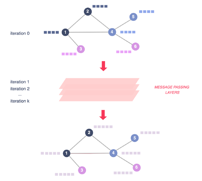
Figure 4 - GNN overall structure, illustration by Lina Faik
What kind of “information” does a node embedding actually encode?
- Structural information about the graph (e.g., degrees of all the nodes in their k-hop neighborhood).
- Feature-based information about the nodes’ k-hop neighborhood.
What is the message passing framework about?
What is a message-passage layer composed of? How are embeddings updated at each iteration? During each message-passing iteration in a GNN, a hidden embedding h_u corresponding to each node u is updated according to information aggregated from u’s graph neighborhood N(u). The figure below illustrates the first iteration.
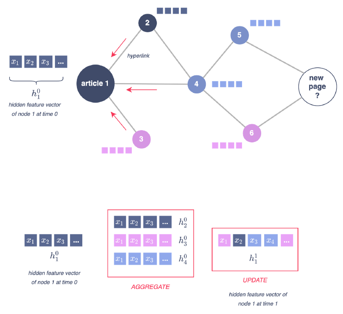
Figure 5 - Illustration of a message passing layer, illustration by Lina Faik
The message-passing update is expressed as follows:
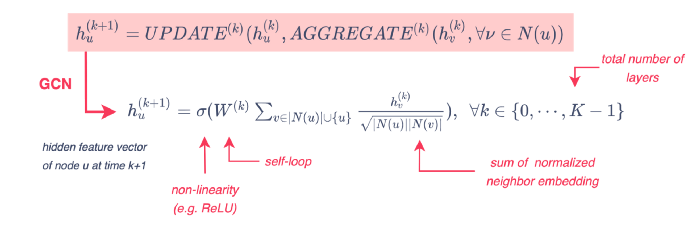 Figure 6 - Message passing function, illustration by Lina Faik
The UPDATE and AGGREGATE functions vary depending on the model. For instance, GCN models rely on a symmetric-normalized aggregation as well as a self-loop update approach as shown in the previous figure.
What is the intuition behind this type of normalization? It provides more importance to neighborhood nodes that are not very connected (low degree). This is relevant for use cases such as the classification of pages as highly connected nodes tend to discuss very broad and general topics. Thus, they do not provide information that is truly useful for classifying the nodes to which they are linked.
GCN approach has proved to be one of the most popular and effective baselines for GNN architectures. How do they relate to the concept of convolution? Just as CNNs aggregate feature information from spatially-defined patches in an image, GNNs aggregate information based on local graph neighborhoods. The figure below illustrates the analogy.
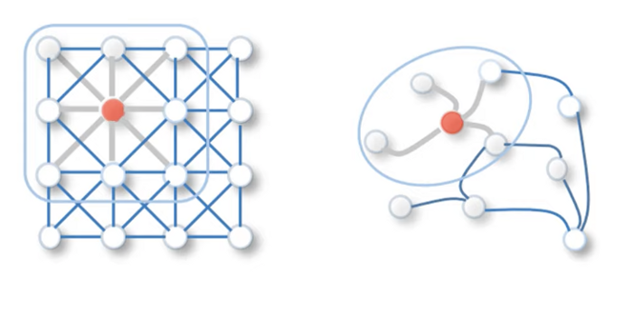
Figure 7 - Analogy between convolutions and the GNN approach, Source
To compare the performance of this approach to traditional machine learning models, I implemented a GCN-based model and compared it to a random forest classifier.
As shown in the code below, the GCN is composed of two graph convolutional layers with a non-linear transformation between them and a final softmax layer for multi-class classification.
The figure below shows the learning curves during the training.
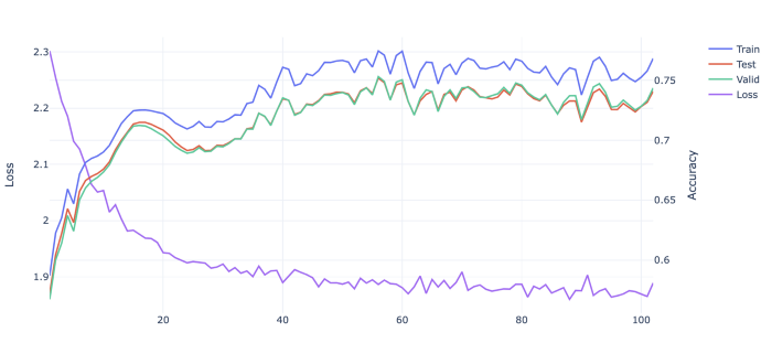 Figure 8 - Evolution of the AUC during the training over the epochs
It is also possible to visualize the evolution of the embeddings as the model is training using t-SNE algorithm as represented in the figure below.
Figure 9 - Evolution of the embeddings during the training
Train / Validation sets. So far, the model is trained and tested on only one split of the initial data. However, the choice of the training split can significantly impact model performance when it comes to node classification. Luckily, the WikiCS dataset provides 20 different training splits, each consisting of 5% of nodes from each class. To ensure a robust comparison, I trained and tested each model on every split.
Hyperparameters. I also tested different combinations of hyperparameters for each model. For more information, you can refer to the code here.
Features. To take the comparison further, I also enriched the dataset used by the random forest by adding graph-related features. These features include nodes degree, triangles, square clustering, clustering, eigenvector centrality, and page rank. For more information about these metrics, you can refer to my previous article here.
As shown in the figure below, GCN tends to learn more efficiently from the data and outperforms the random forest classifier on the validation set. Enriching the dataset by adding graph-related features provides a relatively small improvement in the performance of random forest.
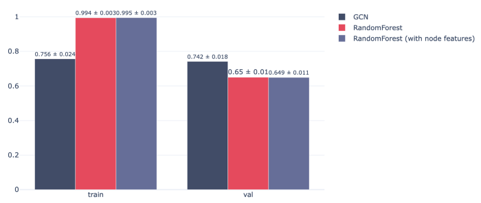
Figure 10 - Performance of models on the train/validation sets in terms of AUC
2.3 Graph Attention Network (GAT)
What are the key concepts behind the model?
GCN models rely on a symmetric-normalized aggregation function that favors nodes depending on their degree. But what if the model could also learn what weight to give to each neighbor during the aggregation step? This can be done by including attention mechanisms in the learning process of the GNN.
The first GNN model to apply attention was Velickovic et al. [2018]’s Graph Attention Network (GAT), which uses attention weights to define the weighted sum of the neighbors:
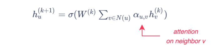
For more about attention, you can read this article from DFTT.
How does the model perform?
The figure below presents the final results. It turns out that the GAT models lead to similar results as GCN for this use case.
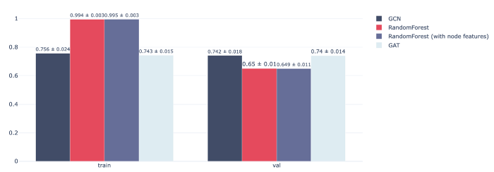 Figure 11 - Performance of models on the train/validation sets in terms of AUC
3. Key Takeaways
GNN frameworks offer a powerful approach by allowing models to learn patterns from graphs that are typically undetectable by traditional ML models. This comparison illustrates the improvement that a simple GCN or GAT model can bring to node classification.
However, depending on the use case and the data that you have, you might opt for one approach over another when carrying out your node classification task:
- Availability of data. Node features (such as the content of the pages) may not be available in other uses cases. And graph-based features that usually reflect nodes’ centrality may not be correlated to the label to predict at all! Thus, graph-based models remain the only relevant option.
- Computing time. GNNs are more expensive than traditional approaches. They take a longer time to be trained. You may be forced to make a trade-off between performance and cost.
- Explainability. The interpretation of the GNN results may not be as straightforward as other models. There are some local approaches that provide an understanding of the reasons that influenced a prediction. But decision trees might be more useful to understand the model as a whole for instance even if it means losing a little in terms of performance.