


In the previous article, we explored the limitations of the conventional search method for data discovery and the need for a join suggestion pipeline. Now, let’s shift our focus to Lazo, the technique employed for the crucial set-matching phase within this pipeline.
To understand Lazo better, it’s essential to grasp the foundational concept of MinHash Local-Sensitivity Hashing (LSH), which serves as the main building block in Lazo’s pipeline. In general, there are two scalability bottlenecks with the naive pairwise similar item searching:
- Comparing large sets involves high computational costs.
- The potential pairs to compare grow exponentially with the total number of items, straining efficiency.
MinHash LSH provides an approximate approach to address these problems:
- Minhashing compresses large sets into concise signatures while preserving Jaccard Similarity.
- LSH identifies pairs of signatures likely to belong to similar sets without necessitating pairwise comparisons.
It’s important to note that this technique does not return a similarity score for every candidate. It returns all potential matches with estimated similarity scores greater than a predefined threshold. Therefore, it is not possible to rank the result without a post-processing step.
The underlying metric supported by MinHash LSH is Jaccard Similarity. However, for the specific use case of join suggestion, our focus will shift to Jaccard Containment — a related yet distinct metric. This distinction underscores the necessity of Lazo (or LSHEnsemble) in this context.
Ideally, the probability of a column being returned as a candidate should have the form of a step curve. This pattern ensures that only good candidates are retrieved — those with Jaccard Similarity exceeding the selected threshold. There are no false negatives and no false positives.
The ideal probability curve with a similarity threshold of 0.6
In the following sections, we will demonstrate that MinHash LSH will indeed approximate this curve.
MinHash
In the context of enterprise data lake environments, sets tend to be very large, often containing thousands of values. The process of storing and comparing such sets can be time-consuming.
To address this, we will replace large sets with more compact representations known as signatures, achieved through hashing. An important attribute of these signatures is their ability to maintain the underlying similarity between the original sets. Each type of distance measurement (Jaccard, Hamming, Cosine, etc.) corresponds to a specific hashing function. Lazo utilizes MinHash, which conserves the Jaccard Similarity, the ratio of the set intersection size over their union size. The probability of a MinHash function producing identical hash values for two sets equals the Jaccard Similarity of those sets:
To generate the signature of each column, we apply multiple MinHash functions. The resulting signature matrix takes the shape (K, C), where K represents the number of hash functions and C is the number of columns within the data lakes.
Why use multiple hash functions? Each row of the signature matrix is an independent observation. The count of rows in which two columns agree equals the expected Jaccard Similarity of their respective sets. Increasing the number of Minhash functions, i.e., augmenting the number of rows in the signature matrix, reduces the expected error in estimating the Jaccard Similarity.
A typical count of hash functions ranges from 128 to 512, significantly smaller than the average set size.
Despite having compact column representations, identifying similar candidates for a query column remains resource-intensive if sticking to a naive pairwise comparison method as its running time scales linearly with the number of columns in the data lake. Hence, the necessity arises for Local-Sensitivity Hashing, an approximative neighbor search technique.
Local-Sensitivity Hashing
Principle
LSH is a technique that builds upon the Minhash signature matrix we discussed earlier. It introduces a process called “banding” where, for each column, several rows (several MinHash values) are grouped into bands, and the combined value within each band is hashed to a bucket.
In querying time, when comparing a pair of columns, a collision occurs if any of their corresponding bands are hashed to the same bucket, indicating similarity between the columns.
When looking for candidates for a query column, we examine its LSH buckets and retrieve other columns hashed into the same buckets as potential candidates. The query time no longer depends on the number of columns in the data lakes but on the number of buckets, which is a much smaller figure. Similarly, the storage costs are optimized as we now solely retain the bucket identifier instead of the actual data it represents. Naturally, this holds true as long as the indexed columns remain unchanged.
The implementation of LSH involves choosing a specific band size denoted as n, which in turn determines the number of bands, represented as b. In the following discussion, we will establish the relationship between these parameters and the probability of a column being returned as a candidate.
Analysis of the Banding Technique
As mentioned earlier, the likelihood of a MinHash function producing the same value for two sets is determined by their Jaccard Similarity, denoted as s.
Within a specific band comprising n rows, the collision probability between two sets is:

This corresponds to the probability that all MinHash values within the band are identical.
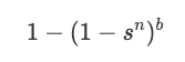
With b bands, the probability of encountering no collisions across any of the bands is:
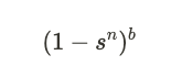
Ultimately, the probability of encountering at least one collision among the bands is given by:
We have thus established the relationship linking the probability of a column being returned as a candidate with the band size n. With this insight, we can effectively determine the optimal parameter for the specific use case.
Parameter Tuning
The function described above has the shape of an S-curve, resembling the desired step curve we initially discussed.
Nevertheless, since it’s not a perfect step function, we can anticipate the presence of both false positives and false negatives. False Positives refer to returned candidates whose Jaccard Similarity falls below the chosen Jaccard Similarity threshold. On the other hand, False Negatives are candidates not returned, despite their Jaccard Similarity exceeding the threshold.
In the example above, the similarity threshold is set at 0.6, which corresponds to the point where the rise is the steepest. However, as shown in the graph, there is still a probability that columns with lower similarity scores might still be returned (False Positives). To illustrate, for columns having a Jaccard Similarity score of 0.5, there is a 20% chance of collision with the query column. The same principle applies to false negatives but in the opposite direction: for columns with a Jaccard Similarity of 0.7, there is a 30% chance of not having any collision with the query column across the buckets. This leads to these columns being left out of the candidate list.
In order to get a curve that reflects our tolerance of False Negative and False Positive rates, we can tune the number of rows n in a band (and thus the number of bands b as they are related together). For example, having few bands with many rows will only get collisions between pairs with a very high Jaccard Similarity. Having many bands with few rows will get collisions between pairs with potentially a very low Jaccard Similarity.
So concretely, how do we achieve this? Given:
- The total number of minhash functions K (equivalent to the number of rows in the signature matrix).
- A chosen Jaccard Similarity threshold S.
- Weights (representing cost of misclassification) assigned to False Negative (wfnr) and False Positive (wfpr) rates.
The optimal band size for that specific similarity threshold can be determined by following these steps:
- Create a list of all potential combinations of the number of bands b and the number of rows in each band n that satisfies the condition (b * n) <= K.
- For each combination, calculate the weighted sum of the False Positive rate and False Negative rate:
- Choose the combination of parameters that results in the smallest error.
In essence, this process allows us to tailor the parameters to strike the right balance between False Positives and False Negatives, providing a configuration that suits the given use case.
Lazo
MinHash LSH is effective at finding neighbors with high Jaccard Similarities (the ratio of the intersection size of sets to their union size). Some of its main applications are similar document search and entity matching. However, this metric is not optimal for join suggestion. In this use case, the goal is to identify candidates with the highest possible overlap with the query set, enabling a potential complete join.
In the example below, candidate 1 (left, red) has a higher Jaccard Similarity with query one (blue), despite candidate 2 having a larger intersection size and probably leading to a more complete join. This behavior arises because JS considers the size of the union between sets, leading to penalties for significant differences in set sizes.
For join suggestion, a more suitable metric is Jaccard Containment, representing the ratio of the intersection size to the size of the query set. However, there are no Local-Sensitivity-family hashing functions that directly support Jaccard Containment. Recent advancements, including Lazo and LSH Ensemble, build upon the Minhash LSH foundation, estimating Jaccard Containment through derived relationships between Jaccard Containment and Jaccard Similarity.
In this article, we will delve into Lazo for two compelling contributions:
- The Lazo paper highlights that the method is more scalable compared to LSH Ensemble, making it more applicable in enterprise scenarios.
- Both Lazo and LSHEnsemble return candidates above a chosen Jaccard Containment threshold. However, only Lazo estimates the actual Jaccard Containment value between the query column and candidates, facilitating candidate ranking.
Establishing the Relationship Between Jaccard Containment and Jaccard Similarity
Let’s begin with an important observation: The highest achievable Jaccard Similarity between two sets occurs when the intersection size is at its maximum, while the union size is at its minimum. This scenario reflects one set entirely encompassing the other (depicted on the left), where the intersection size is the size of the smaller set, and the union size is the size of the bigger set:
On the other hand, the lowest Jaccard Similarity between two sets is zero, emerging when their intersection set is completely empty (shown on the right).
Transitioning from JSmax(X,Y) to JSmin(X,Y) involves adding “α” elements from the intersection set into the union set. This process visually resembles pulling apart two circles: their intersection reduces while their union grows. This series of observations lead us to the final expression of Jaccard Similarity:
The same reasoning can be applied to Jaccard Containment:
Hence, to estimate the Jaccard Containment, we must determine α, which can be calculated using the following equation (derived from the earlier expression):
In this context, three values require estimation:
- The cardinality of sets X and Y.
- The Jaccard Similarity between sets X and Y.
To address this, HyperLogLog is a readily available technique to estimate cardinalities efficiently.
However, as underlined in the previous part, MinhashLSH does not provide the estimated Jaccard Similarity, necessitating an inference mechanism. This is where Lazo’s second contribution comes into play.
Estimating Jaccard Similarity From MinHashLSH
Recall that MinHashLSH is a probabilistic technique designed to retrieve candidates with Jaccard Similarity greater than a predefined threshold. However, it doesn’t provide the estimated score for each candidate, leaving us with two options. The first approach involves explicitly calculating the Jaccard Similarity for each candidate, which is both resource-intensive and time-consuming.r
Otherwise, a simple approximation approach is to index the data into multiple LSH indexes, each with a different similarity threshold. When querying, the highest threshold at which a column becomes a candidate can be considered its estimated Jaccard Similarity. This is still costly regarding storage and running time as the number of LSH buckets grows linearly with the number of thresholds used.
Following the same principle, Lazo introduces a small strategy to circumvent this multiplication of hash buckets. Given the list of similarity thresholds, we can determine the necessary band sizes using the approach outlined in Part 3. Subsequently, identifying the greatest common divisor among these band sizes yields the unit band size essential for indexing.
This unit band size corresponds to one of the lower thresholds. When querying for higher thresholds, their bands will encompass several unit bands, each stored in a separate bucket. Lazo’s strategy then involves querying these individual buckets and aggregating outcomes through intersections. This strategy retains the straightforwardness of the earlier approximation approach while avoiding the necessity for an excessive multiplication of hash buckets.
Consider the below signature matrix:
Assuming:
- The unit band comprises two MinHash values.
- The chosen similarity threshold requires a band size of four, equating to two unit bands.
During the first iteration, Lazo fetches the first two bands. Candidates are identified through collisions occurring in both bands (hence the intersection operation). If the second column serves as the query, the candidate corresponds to the last column (as shown in the graph where the same color signifies the same values).
Conclusion
In summary, Lazo introduces an interesting technique based on MinHashLSH, tailored to excel in join suggestion scenarios. It accomplishes this by focusing on Jaccard Containment, aligning seamlessly with our use case. Lazo’s contributions come in two main parts: First, it establishes a mathematical relationship between Jaccard Containment and Jaccard Similarity. Second, it proposes an effective strategy to estimate Jaccard Similarity without exploding the number of hash buckets to store. This makes Lazo an essential tool for streamlined data analysis, demonstrating its usability and effectiveness in the ever-changing enterprise data landscape.