There is a clear trend in the data science and machine learning industry on training bigger and bigger models. These models achieve near-human performance, but they are usually too big to be deployed on a device with constrained resources like a mobile phone or a drone. This is one of the main blockers to the broader adoption of AI in our everyday lives.
How can I fit my 98Mb ResNet model in a 15Mb mobile app?
On Android, the average app size is 15Mb, whereas NASNet, a state of the art image classification model released by Google, achieves over 80% accuracy on ImageNet — a famous image classification competition — but has a 355Mb size in its large version and 21.4Mb in its mobile-optimized version.
If you’re a data scientist trying to fit high-performing models into devices with constrained resources, this article will give you practical tips on how you can compress your model size by up to 70% with Keras and NumPy only, without losing performance.
In the last few years, there has been a lot of interest in making models smaller for resource-efficient training and inference on such constrained devices. Two main approaches have been used:
The first and most popular method is to train neural networks that are lightweight by design. A good example of this is MobileNet by Google. MobileNet’s architecture only features 4.2 million parameters while achieving a 70% accuracy on ImageNet. This compression maintains reasonable performance and is achieved by the introduction of depth-wise convolution layers which help reduce model size and complexity.
The other type of approach is to leverage large, pre-trained neural networks and compress them to reduce their size while minimizing loss in performance. This article will focus on reviewing and implementing some of these compression techniques on convolutional neural networks (CNNs).
In particular, we will focus on pruning techniques, the low hanging fruit of neural network compression. Network pruning aims at removing specific weights and their respective connections in a neural network to compress its size. Although pruning is less popular than other approaches, it achieves pretty good results and is quite easy to implement, as we will see in the rest of this article.
“The ability to simplify means to eliminate the unnecessary so that the necessary may speak.” Hans Hoffman
It might seem odd that removing weights from a neural network wouldn’t drastically harm its performance. Still, in 1991, Y. LeCun et al. showed in a paper called Optimal Brain Damage that one could reduce the size of a neural network by selectively deleting weights. They found it was possible to remove half of a network’s weights and end up with a lightweight, sometimes better-performing network.
In the particular case of CNNs, instead of removing individual weights, most approaches focus on removing entire filters and their corresponding feature maps from convolutional layers. The main benefit of this method is that it doesn’t introduce any sparsity in the network’s weight matrices. This is important to take into account as most deep learning frameworks, including Keras, don’t support sparse weight layers.
Although convolution layers only account for a minority of the network’s weights — the bulk of the network is in the fully connected layers — pruning filters eventually reduces the number of weights in the dense layers.
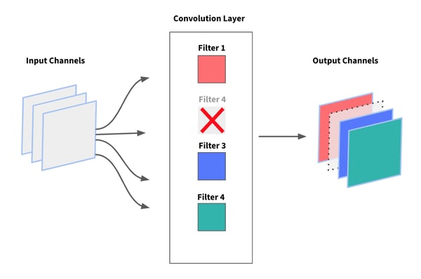 Pruning convolution filters from CNNs
What Is the Intuition Behind Network Pruning ?
Let’s take a step back for a second and look at the intuition behind network pruning. There are two hypotheses on neural networks that motivate pruning:
The first one is weight redundancy. This means that several neurons — or filters in the particular case of CNNs — will be activated by very similar input values. Consequently, most networks are actually over-parameterized and we can safely assume that deleting redundant weights won’t harm performance too much.
The second one is that not all weights contribute equally to the output prediction. Instinctively, we can assume that lower magnitude weights will have a lower importance to the network, Y. LeCun calls them low saliency weights. Indeed, all things being equal, lower magnitude weights will have a lower effect on the network’s training error.
As we can see in the figure below, a large number of the convolution filters across the network have a low L1 norm while a very small number of filters have a much larger norm.
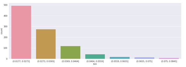
Distribution of L1 norm of filters on all layers of a CNN trained on imagenette
Although using L1 norm is a simplistic heuristic to rank the importance of filters, we can assume that pruning low importance convolution filters away from the network would have a lesser impact than others.
Now that we have a better understanding of pruning and how it can help compress networks without harming their performance, let’s see how we can implement it on a Keras network.
How to Prune a Model Trained With Keras?
In the remainder of this article, we’ll use a vanilla CNN trained on imagenette, a subset of 10,000 images from 10 ImageNet categories. After training and evaluating our full baseline network, we’ll implement and compare different pruning strategies.
Rank-Prune-Retrain
The algorithm we will adopt to efficiently prune our CNN is surprisingly simple: Rank — Prune — Retrain. First, we’ll need to rank our filters by importance in order to identify low magnitude, unimportant filters. Then, we’ll prune away a certain percentage of them based on their estimated importance. Finally, we’ll retrain the network for a few epochs using the same learning rate as for the initial training to fine-tune weights to the new pruned architecture. That’s it, it’s so simple it can fit in one Tweet.
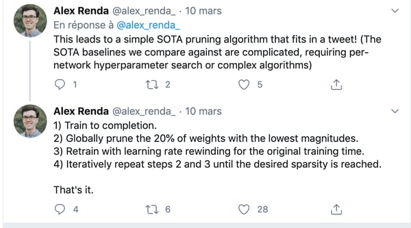
The NN compression algorithm by Alex Renda
- Rank: Identifying Filters to Prune
There is no consensus on how to rank weights according to how much they contribute to the output performance of the network. A perfect strategy would be to prune each weight individually and compute the performance of the model without the weight. This method is called oracle pruning, but with several millions (sometimes billions) of weights in a network, it is a very expensive strategy to say the least.
Other proxies to rank weights involve computing their norm (L1 or L2) or computing the mean, standard deviation or percentage of 0 activation values over a batch of input data.
For this experiment, we’ll use both L1 norm and Average Percentage of Zero (APoZ) Activations of the convolutional filters to rank them by importance.
Since we’re going to use L1 norm to compare filters with different sizes, we’ll have to use a normalized L1 norm:
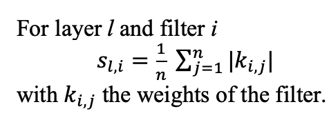
The code below computes L1 norm of the convolutional filters in a Keras model and outputs a matrix of dimension Nb_of_layers x Nb_of_filters.
The second option you can try is to compute the APoZ activations. The intuition is that if a filter is rarely activated over a batch of random input images, it doesn’t contribute much to the output predictions of the model. Note that this metric makes a lot of sense if the activation functions used in the convolutional layers zero out a lot of values. This is the case for ReLU but when using other functions like Leaky ReLU, the APoZ criteria might not be as relevant.
To compute APoZ per filter, we’ll have to select a subset of the dataset, score it with our CNN, and compute each filter’s average percentage of activation values equal to 0. The filters we will prune are the ones with the biggest percentage of zero activations.

The following function does that for one convolutional layer:
Generalizing that to all layers, again, we’re outputting a Nb_of_layers x Nb_of_filters matrix with an APoZ value for each individual filter in the network:
From these two matrices, we can easily identify which filters to prune. Some papers set a hard threshold and prune away all the filters that don’t make the cut, while others rank the filters and set a target percentage of filters to prune away.
In the code below, we are pruning away 10% of the filters in the network by simply computing the number of filters n_pruned corresponding to 10% of the filters and then computing coordinates of the n_pruned lowest (for L1) or biggest (for APoZ) values in the matrix:
In addition to these two methods, we also tried pruning away random filters from the network to prove that you can’t just remove random filters from the network and get away with it!
2. Prune: Pruning Away the Filters
Now that we have identified the convolutional filters to remove, we’ll have to put on our brain surgeon hat and delete the filters from the network. We’ll also need to be cautious and remove the corresponding output channels in the deeper layers of the network.
Thankfully, the keras-surgeon library provides very simple methods to efficiently modify trained Keras models. Building on the simplicity of Keras, keras-surgeon lets you easily delete neurons or channels from layers using a simple delete_channels_method(). The library also has an identify module that lets you compute the APoZ metrics for neurons in a specific layer. Keras-surgeon is awesome and works on virtually any Keras model (not just CNNs) — shout out to Ben Whetton for his work on this. Here’s the link to the repo.
Let’s implement keras-surgeon to prune away the channels identified in the previous section. We’ll also have to re-compile the model once it’s been pruned using the standard .compile() module in Keras.
We can wrap this up with a nice prune_model() function.
During our experiment, we tried different pruning percentages, pruning up to 50% of the convolution filters in the network. This revealed that after a certain point, we removed too many essential filters from the network and the drop of performance was too big to be recovered by further fine tuning.
The best pruning — performance ratio was achieved by pruning away 20% of the filters using APoZ, which enabled us to reduce the number of model weights by 69%!
3. Retrain: Retraining the Model
Our model is now stripped of a good chunk of the allegedly unnecessary filters. Pruning the model introduced perturbations in the model and, in order to maintain the model’s performance, it is usually necessary to fine-tune the model for a few epochs. Keras makes it very easy to fine-tune a previously trained model, simply call the .fit() function again using the same optimizer (same optimizer type, same learning rate) as the initial model training.
The amount of fine-tuning to be done will depend on the proportion of filters pruned from the model and the initial model complexity. For our experiments, we chose to retrain for one epoch only on our vanilla CNN, but some papers use up to 10 epochs of retraining on more complex models.
Something interesting to note is for models pruned using L1 and APoZ, the performance actually increased compared to the baseline after pruning and retraining them. Our network, despite being 69% smaller in size, has a 77.8% accuracy, much better than our baseline, over-parameterized model, which is very cool to see.
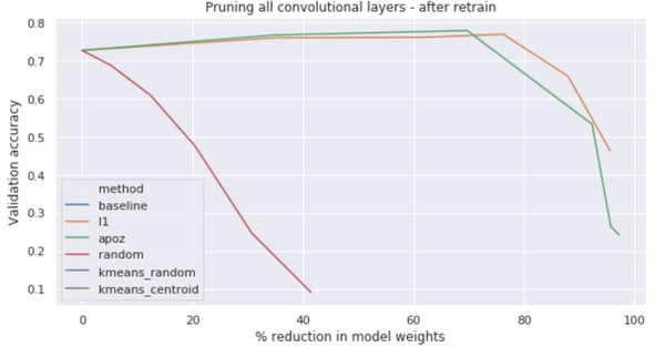
Evolution of model performance at increasing pruning % (in number of model weights) using L1, APoZ and random pruning of filters.
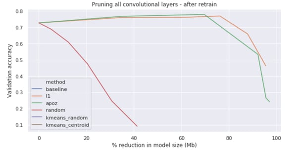
Evolution of model performance at increasing pruning % (in model size) using L1, APoZ and random pruning of filters.
This has been observed in several papers and can be interpreted as a post-training network regularization. Even if you’re not looking to compress your model, you might want to have a go at pruning as a way to improve its generalization performance.
4. Repeat!
This Rank — Prune — Retrain cycle can be repeated iteratively until a certain criterion is met. For example we could repeat this cycle until the difference between the pruned model’s performance and the original model’s performance is bigger than a certain threshold.
In practice, we found that a single iteration of this cycle could lead to up to a~70% compression in number of weights while maintaining or improving the performance of our baseline CNN.
Conclusion
To conclude on these experiments, we saw that APoZ gave slightly better compression / performance results than L1. However, in practice, I’d suggest using L1 as a quick win for compression. As opposed to APoZ, L1 doesn’t require any data to identify filters to prune and is thus much less computationally intensive than APoZ.
Overall, we’ve been impressed by the compression results achieved using such a conceptually simple technique. Compared to other compression techniques like quantization, pruning is a much simpler approach to implement while producing very nice results. It is our hope that this article convinced you to give pruning a try and that we’ll see more pruned models being deployed to production!
