


Last time, we learned about curiosity in deep reinforcement learning. The idea of curiosity-driven learning is to build a reward function that is intrinsic to the agent (generated by the agent itself). That is, the agent is a self-learner, as he is both the student and its own feedback teacher.
To generate this reward, we introduce the intrinsic curiosity module (ICM). But this technique has serious drawbacks because of the noisy TV problem, which we’ll introduce here.
So today, we’ll study curiosity-driven learning through random network distillation used in the paper Exploration by Random Network Distillation, and you’ll learn how to implement a PPO agent playing Montezuma’s Revenge with only curiosity as reward. Let’s get started!
The Problem With the Prediction-Based Intrinsic Reward: Procrastinating Agents
Last time, we learned that one of the solutions to sparse rewards is to develop a reward function that is intrinsic to the agent. This intrinsic reward mechanism is known as curiosity because it will motivate our agent to explore the environment by going to states that look novel or unfamiliar.
In order to do that, our agent will receive a high reward when exploring new trajectories. But ICM generates curiosity by calculating the error of predicting the next state given the current state, and this leads to a big problem: procrastinating agents.
Remember that reinforcement learning is based on the reward hypothesis; that is, each goal can be described as the maximization of the expected cumulative reward. Consequently, the agent (in order to have an optimal policy) must select the actions that will maximize its rewards.
For next-state-prediction agents, the reward is the prediction error. Therefore, our agent wants to explore the environment since this will favor high prediction error transitions.
But here’s the problem: because of the way we calculate the intrinsic reward, by predicting the next-state, our agent can fall into what we call the Noisy TV problem. Noisy TV problems show how next-state prediction agents can be attracted by stochastic (random) or noisy elements in the environment.
Let’s say you have a noisy TV in the environment that displays new images in unpredictable order. This is a source of stochasticity that causes every next state to be unpredictable.
 Our agent will stay in front of this stochastic element. GIF adopted from a video (taken on Google AI blog) by Deepak Pathak, used under CC BY 2.0 license.
It means that at every timestamp, the curiosity reward will be high because it will be very hard to predict the next state (since the next state is random).
This leads to procrastination-like behavior: our agent, in order to maximize its rewards, will stay in front of this noisy TV instead of doing something useful. Indeed, our agent will always experience high intrinsic reward, as he will be unable to correctly predict the next-state because of this stochastic element in the environment.
We can also see in the Google AI experiment that instead of exploring the labyrinth, the agent prefers to shoot the wall because he’s not able to predict the animation on the wall, and thus he obtains high rewards.
 The agent shoots on the wall to maximize its rewards.
How we can solve this problem?
A solution is to develop a method that calculates curiosity but that is not attracted by the stochastic elements of an environment. This is exactly what the exploration by random network distillation (RND) method proposes.
Curiosity Through Random Network Distillation (RND)
Within an RND, we have two networks:
- A target network, f, with fixed, randomized weights, which is never trained. That generates a feature representation for every state.
- A prediction network, f_hat, that tries to predict the target network’s output.
Because the target network parameters are fixed and never trained, its feature representation for a given state will always be the same. Instead of predicting the next state s(t+1) given our current state s(t) and action a(t) as for ICM, the predictor network predicts the target’s network output for the next state.
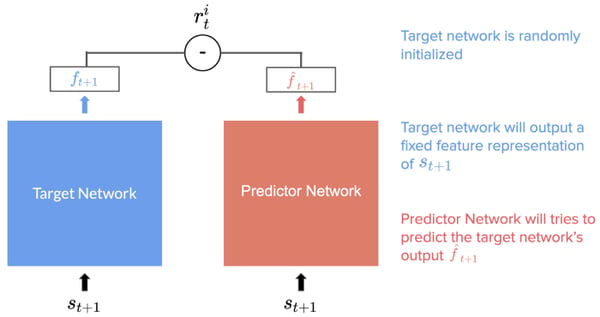
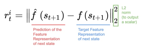
Therefore, each state s(t+1) is fed into both networks, and the prediction network is trained to minimize the difference mean square error (between the target network’s output and the predictor network’s output). This is denoted by r in these formulas.
This is yet another prediction problem: our random initialized neural network outputs are the labels, and the goal of our prediction is to find the correct label. This process distills a randomly initialized neural network (target) into a trained (predictor) network.
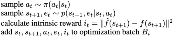
If we go back to the Markov decision process formulation, we add a new step to calculate the intrinsic reward:
 Source: Exploration by random network distillation
- Given the current state s(t), we take an action a(t) using our policy π
- We get the extrinsic reward r_e(t) and the next state s(t+1)
- Then we calculate the intrinsic reward ri(t) using the formula above
Some Shared Similarities With ICM
Just like for ICM, when reaching previously visited states, the RND agent receives a small intrinsic reward (IR) because the target outputs are predictable, and the agent is disincentivized to reach them again. And when in an unfamiliar state, it makes poor predictions about the random network output, so the IR will be high.
 Source: Exploration by random network distillation
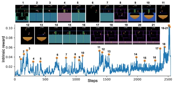
We can see on the experimentation of OpenAI on Montezuma’s Revenge that the spikes in the IR (or the prediction error) correspond to meaningful events:
- Losing a life (2, 8, 10, 21)
- Escaping an enemy by a narrow margin (3, 5, 6, 11, 12, 13, 14, 15)
- Passing a difficult obstacle (7, 9, 18)
- Picking up an object (20, 21).
This implies that intrinsic reward is non-stationary: what’s new at a given time will become usual through time, as it will be visited more and more during training. This will have some consequences when we’ll implement our agent.
Overcoming Procrastination
Contrary to ICM, the RND agent no longer tries to predict the next state (the unpredictable next frame on the screen), but instead the state’s feature representation from the random network. By removing the dependence on the previous state, when the agent sees a source of random noise, it doesn’t get stuck.
Why? Because after enough training of states coming from stochastic elements from the environment (random spawning of objects, random movement of an element, etc.) , the prediction network is able to better predict the outputs of the target network.
As the prediction error decreases, the agent becomes less attracted to the noisy states than to other unexplored states. This reduces the Noisy-TV error.
But more importantly, beyond this theoretical concern (after all, most of our video game environments are largely deterministic), RND provides an architecture that is simpler to implement and easier to train than ICM since only the predictor network is trained.
While the noisy-TV problem is a concern in theory, for largely deterministic environments like Montezuma’s Revenge, we anticipated that curiosity would drive the agent to discover rooms and interact with objects.
Implementation
Our PyTorch implementation is a modification jcwleo’s work. I modified the code and commented each part in order to be comprehensive. You can find it here. We trained this agent for 21 hours with 128 parallel environments in a Tesla K80 (we give you the saved models, they are in the github repo). Ultimately, we reached the score of 3800 and discovered 6 rooms.
The RND Model
We used:
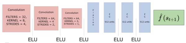
- Predictor: A series of 3 convolutional layers and 3 fully connected layers that predict the feature representation of s(t+1).
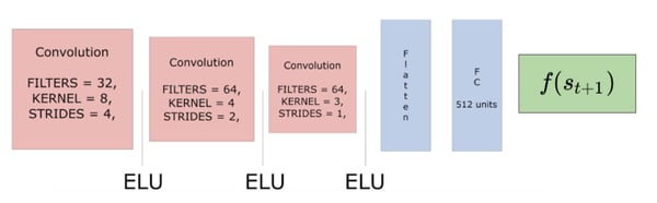
- Target: A series of 3 convolutional layers and 1 fully connected layer that outputs a feature representation of s(t+1).
Combining Intrinsic and Extrinsic Returns
In ICM, we used only IR — treating the problem as non-episodic resulted in better exploration because it is closer to how humans explore games. Our agent will be less risk averse since it wants to do things that will drive it into secret elements.
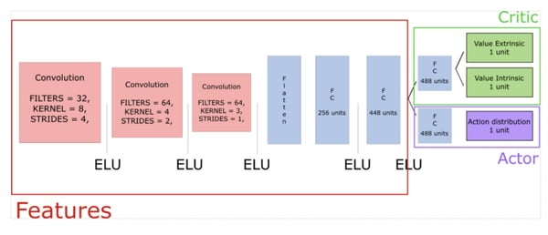
Two Value Heads
Our new PPO model needs to have two value function heads: because extrinsic rewards (ER) are stationary whereas intrinsic reward (IR) are non-stationary, it’s not obvious to estimate the combined value of the non-episodic stream of IR and episodic stream of ER.
The solution is to observe that the return is linear i.e R = IR + ER. Hence, we can fit two value heads VE and VI and combine them to give the value function V = VE + VI. Furthermore, the paper explains that it’s better to have two different discount factors for each type of reward.
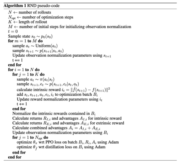
Reward and Observation Normalization
Reward normalization: One of the challenges in this model is that the intrinsic reward decreases as more states become familiar and might vary between different environments, making it difficult to choose hyperparameters. To overcome this, the intrinsic rewards are normalized in each update cycle by dividing it by a running estimate of the standard deviation of the intrinsic returns.
Observation normalization: Going without it can result in the variance of the embedding being extremely low and carrying little info about the inputs. Consequently, we whiten each dimension by subtracting running mean then dividing by the running standard deviation and finally, clipping the norm observation between [-5,5].
But first, we initialize the norm parameters by stepping a random agent in the environment for small number of steps before beginning optimization — we use that for both predictor and target networks.
To conclude, RND was able through exploration to achieve very good performance. But there is still a lot of work to be done. As explained in the paper, RND is good enough for local exploration (exploring the consequences of short term decisions such as avoid skulls, take keys etc). But global exploration is much more complex than that. And long relations (for instance, using a key that was found in the first room to open the last door) are still unsolved. This requires global exploration through long-term planning. Consequently, next time we’ll see another curiosity learning method developed (of course) by Google Brain and DeepMind… stay tuned!