


The most famous implementation of Gradient Boosting algorithm is probably XGBoost [1] for its wins in many Kaggle competitions. Although it performs very well on various tasks, it presents some limits with scalability. Recently, contenders such as LightGBM [2], HistGradientBoosting, and CatBoost [3] have been developed, and they each come with their own implementation tricks to tackle this issue. In the midst of all these possibilities, a question naturally arises: which gradient boosting algorithm is best suited for a given dataset?
To try answer this question, we’ll review the differences between these implementations regarding tree-building strategies and study their impact on scalability and performance.

Does One Implementation Stand Out?
Let’s jump straight to the conclusion of our experiments and present our results ! We’ll follow through with a presentation of the various implementations as promised.
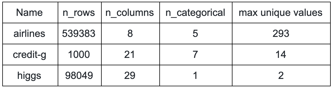
We compare the different algorithms on three datasets: airlines, credit-g and higgs. Here is a summary of their main statistics:
To make the comparison fair and sound, every technical improvement implemented in the libraries is enabled, although some of them will not be addressed in this post. In particular, the native support of categorical features available in LightGBM and CatBoost is used.
The experiment consisted in running a cross-validated, randomized search to optimize the parameters of the different classifiers and measure the mean training time and best test score values reached.
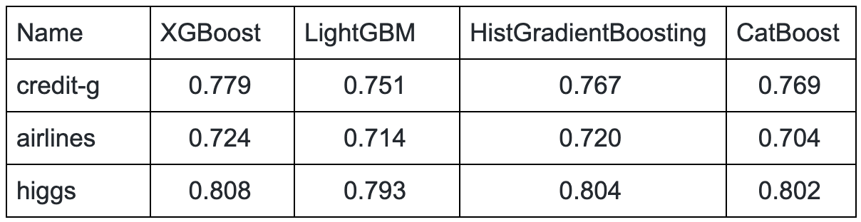
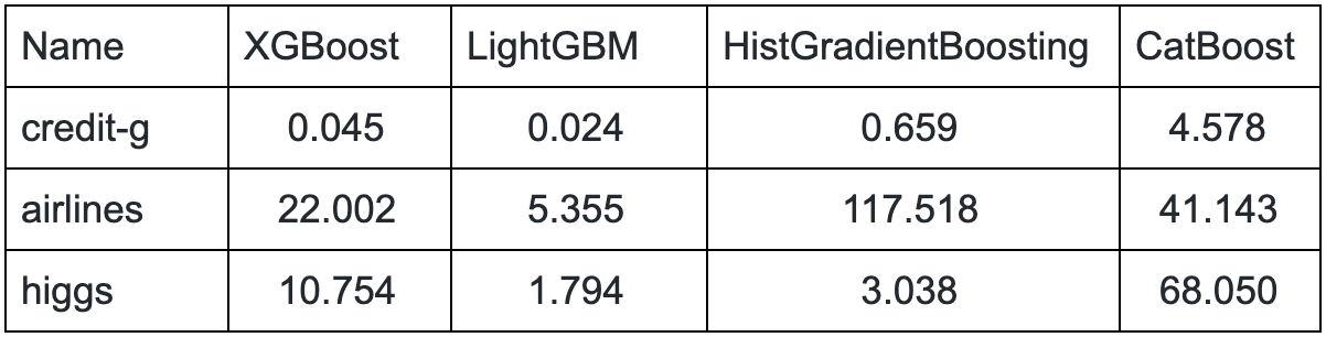
We report the results in tables 2 and 3 below. The different implementations achieve equivalent scores on each of the datasets. However, there are notable differences in the training time:
- LightGBM is significantly faster than XGBoost on every task.
- HistGradientBoosting is very slow on airlines, but does better than XGBoost on higgs. It seems that the algorithm does not handle many one-hot encoded features well.
- Surprisingly, CatBoost is not competitive on this selection of dataset, always outperformed by at least one implementation.
Takeaways for the Impatient reader
Based on our findings, it seems recommended to set the tree method of XGBoost to hist when dealing with large datasets, as it decreases the training time a lot without affecting the performance.
LightGBM is definitely an alternative worth considering, since it was faster and performed equally well on the datasets we studied. The user should not hesitate to use the built-in categorical feature handler.
However, its scikit-learn counterpart HistGradientBoosting — which for the moment, does not come with a similar handler — suffers from poor scalability with a number of columns that does not go well with one-hot encoding.
CatBoost offers an interesting solution to tackle the problem of prediction shift, which was never addressed by previous gradient boosting algorithms. Unfortunately, it was found to be significantly slower than other algorithms on the datasets we tested without offering a real performance boost.
A Closer Look into Tree-building Strategies
A Quick Reminder on Gradient Boosting of Decision Trees
Gradient Boosting of Decision Trees is an ensemble method of weak learners. Each step of the algorithm builds a decision tree that aims at compensating for the prediction errors of its predecessors by fitting the gradient of these errors.
Tree building is done iteratively. Starting from the current node, the algorithm searches for a threshold value that maximizes the information gain of the resulting split. Finding an optimal split for a feature requires going through all data instances in the current leaf. This has to be performed at every split step, for every feature, and every iteration of the algorithm. It rapidly becomes costly in time as the size of the dataset increases.
Recent gradient boosting libraries implement various split-finding techniques to improve scalability that we’ll present now.
Saving Computations by Using Histograms
The first approach, now adopted by every algorithm, is the use of feature histograms when searching for a split point. The idea is to group the values taken by a feature into a pre-set number of bins that approximates the feature’s distribution. The split-finding step then consists in going through every bin of every feature histogram, reducing the complexity of the task from O(#instances × #features) to O(#bins × #features).
Histogram aggregation was only added in a later version of XGBoost, notably after the successful implementation of LightGBM. This method is the main feature of HistGradientBoosting and is also implemented in CatBoost.
Harnessing Gradient Statistics: The Weighted Quantile Sketch
Weighted Quantile Sketch is an exclusive feature of XGBoost. It is an approximate split-finding method that makes use of gradient statistics.
Instead of reading through all data instances, it uses quantiles to define candidate split points. However, candidates are not evenly distributed across the feature values: quantiles are weighted to favor the selection of candidates with high gradient statistics (that is, instances with important prediction error).
Finding the candidate split points is still expensive when the number of data instances is significant. With Weighted Quantile Sketch, one of the contributions of XGBoost is also to design a distributed algorithm that solves this problem in a scalable way.
Which Tree Method Offers the Best Scalability in XGBoost?
The previously described method is referred to as approx in XGBoost API, and the traditional split finding algorithm is denoted by exact. The enhancement of Weighted Quantile Sketch using histograms is now available as hist.
We compared the performance of these three methods on subsamples of different sizes of the Airlines dataset. This dataset is large enough to study how the algorithms scale with the sample size and has categorical variables with high cardinality, that produce many dummy variables after one hot encoding.
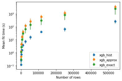
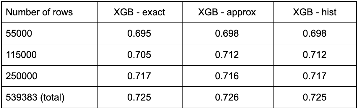
As expected, the use of histograms results in an important speed up in the fit time. However, it appears that the approx tree method is slightly slower than exact on this particular dataset. Regarding the performance, the choice of the tree method does not seem to affect the accuracy of the prediction on the airlines dataset.
The LightGBM Counterpart: Gradient-Based One-Side Sampling
Gradient-Based One-Side Sampling (GOSS) starts from the observation that some data instances are very unlikely to be good candidates for split point and that searching a well-chosen subset of the training set should save computation time while not affecting efficiency.
More specifically, points with higher gradients in absolute value tend to have a higher contribution to the computation of the information gain, and we should prioritize them when sampling from the data. However, exclusively sampling instances with larger gradients would have a negative impact on training, as it would shift the data distribution at every split. This is why GOSS proceeds as follows:
- Instances are ordered according to their gradients absolute value (best first).
- A ratio a of the best samples from the training set is selected (a in [0,1], is set in advance).
- A ratio b of the remaining set is selected (b in [0,1], is set in advance).
- In the computation of the information gain, gradients of samples from step 3 are given a weight factor (1- a)/b to compensate for the bias introduced in sampling.
In the original paper [2], the authors prove that the error made by the approximation of the information gain asymptotically approaches 0 for a balanced split, making the method efficient for large datasets.
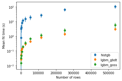
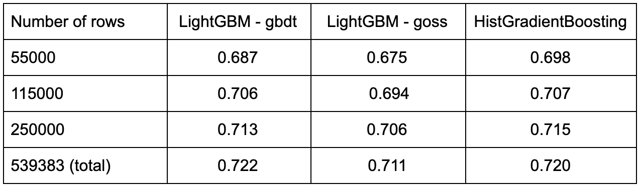
How Does GOSS Compare to GBDT?
Although experiments presented in the paper show that the use of GOSS leads to a significant speed up in training time compared to the GBDT version, we could not reproduce these results with the Airlines dataset.
Instead, it seems that GOSS is slightly more costly in training time. We also included HistGradientBoosting in the experiment, as it is directly inspired by LightGBM. It appears that HistGradientBoosting is always slower than the original LightGBM implementation but still manages to reach comparable performance scores.
The Fresh Angle of CatBoost with Ordered Boosting
In addition to histogram-based split finding, CatBoost formalizes and addresses another problem inherent to gradient boosting. In the paper, authors prove that using training samples both for the computation of the residuals and the construction of the current model introduces a bias in the future predictor, referred to as prediction shift.
The purpose of Ordered Boosting is to reduce this bias, by maintaining a series of models trained on different subsets of the training dataset. For a given permutation σ of [1,n], and a given training dataset D, let us define Dⱼ = { xᵢ ∈ D | σ(i) < σ(j)}. In this way, we define a series of growing subsets of D such that xⱼ is never in Dⱼ. The algorithm maintains a set of models Mⱼ trained on Dⱼ, and the residual of xⱼ is always computed using the prediction given by Mⱼ.
In practice, the algorithm stores the predictions Mⱼ(xᵢ) for i, j ∈ [1,n], rather than the complete models. These predictions are updated at each training iteration after building the new tree.
For a more detailed presentation of the method and other implementation tricks we cannot cover here, do not hesitate to have a look at the original paper. For now, let’s see how ordered boosting compares to the plain setting.
Does Ordered Boosting Affect Scalability and Performance?
We set up a same small experiment to investigate the added value of ordered boosting both in terms of performance and training time. Enabling ordered boosting resulted in an increase of the fit time with no real improvement in accuracy for this particular task.
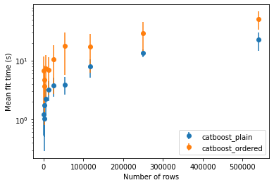
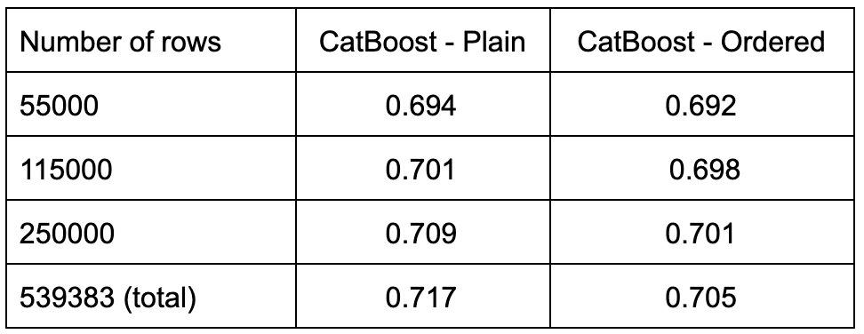
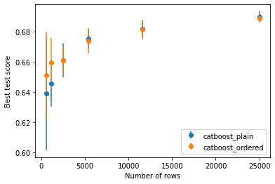
The official recommendation from the authors is to enable ordered boosting when the dataset is small as the prediction model is more likely to overfit. We tried to verify this statement by repeating the experiment several times on different small subsets of Airlines. The results are presented in the figure below: on average, ordered boosting did perform better on subsets of small size.
That wraps up our review of tree-building strategies in gradient boosting of decision trees. In the next post, we will explore existing categorical feature handling methods and their effect on scalability and performance of the algorithms, stay tuned!
References
[1] Chen, T. & Guestrin, C. XGBoost: A scalable tree boosting system. Proc. ACM SIGKDD Int. Conf. Knowl. Discov. Data Min. 13–17-Augu, 785–794 (2016).
[2] Ke, G. et al. LightGBM: A highly efficient gradient boosting decision tree. Adv. Neural Inf. Process. Syst. 2017-Decem, 3147–3155 (2017).
[3] Prokhorenkova, L., Gusev, G., Vorobev, A., Dorogush, A. V. & Gulin, A. Catboost: Unbiased boosting with categorical features. Adv. Neural Inf. Process. Syst. 2018-Decem, 6638–6648 (2018).