Arguably more famous today than Michael Bay’s Transformers, the transformer architecture and transformer-based models have been breaking all kinds of state-of-the-art records. They are (rightfully) getting the attention of a big portion of the deep learning community and researchers in Natural Language Processing (NLP) since their introduction in 2017 by the Google Translation Team.
 Yet another pun on Attention
This architecture has set the stage for today’s heavy-weight models: Google AI’s BERT (and its variants) have been sitting in first position across many NLP leaderboards. OpenAI’s GPT2 was judged so powerful by its authors, that up until recently only a weaker version of it was publicly released, following expressed concerns that this model might be used for “evil”! You can appreciate this claim by yourself.
In this blogpost series, we will walk you through the rise of the transformer architecture. Our first stop will be a focus on the attention mechanism, which is the key component of this architecture. We will then move on to the transformer itself in part II, and finally, we’ll introduce BERT in part III.
Let’s Take a Step Back
In order to understand the transformer and its motives, we will need to dive into its core idea: a novel paradigm called attention. This paradigm made its grand entrance into the NLP landscape (specifically in translation systems) in 2014, well before the Deep Learning hype, in an iconic paper by Bahdanau et. al “Neural Machine Translation by Jointly Learning to Align and Translate.” Before going any further, let’s recall the basic architecture of a machine translation system.

Encoder-Decoder architecture
It follows a typical encoder-decoder architecture, where both the encoder and decoder are generally variants of RNNs (such as LSTMs or GRUs). The encoder RNN reads the input sentence one token at a time. It helps to imagine an RNN as a succession of cells, one for each timestep. At each timestep t, the RNN cell produces a hidden state h(t), based on the input word X(t)at timestep t, and the previous hidden state h(t-1). This output will be then fed to the next RNN cell.
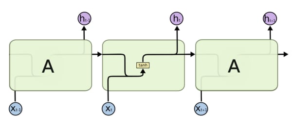 From the amazing seminal post
Eventually when the whole sentence has been processed, the last-generated hidden state will hopefully capture the gist of the all the information contained in every word of the input sentence. This vector, called the context vector, will then be the input to the decoder RNN, which will produce the translated sentence one word at a time.
I can already see that you are a bit skeptical, so let’s get right down to the problem here: is it safe to reasonably assume that the context vector can retain ALL the needed information of the input sentence? What about if the sentence is, say, 50 words long? No. This phenomenon was aptly dubbed the bottleneck problem.
Enters Attention
So how can we avoid this bottleneck? Why not feed the decoder not only the last hidden state vector, but all the hidden state vectors! Remember that each input RNN cell produces one such vector for each input word. We can then concatenate these vectors, average them, or (even better!) weight them as to give higher importance to words — from the input sentence — that are most relevant to decode the next word (of the output sentence). This is what attention is all about.
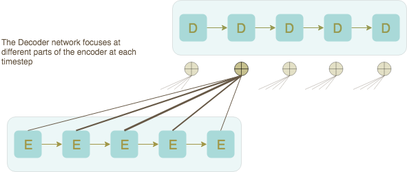
As per the tradition now, this paradigm was in fact first leveraged on images before being replicated on text. The idea was to shift the focus of the model on specific areas of the image (that is, specific pixels) to better help it in its task.
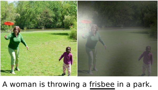 An Image Captioning application: In order to generate the next word in the caption, the model shifts its attention on relevant parts of the image.
The same idea applies to translating text. In order for the decoder to generate the next word, it will first weigh the input words (encoded by their hidden states) according to their relevance at the current phase of the decoding process.
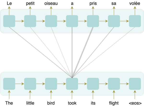 In order to generate the word "took," the decoder attends heavily to the equivalent French word "pris" as well as the word "a," which set the tense of the verb.
Attention Inner Workings
The rest of this article will now focus on the inner-workings of this mechanism. We now know that in order to generate the next word of the output sentence, the decoder will take the previously generated word as input as well as an attention-based weighted sum of all the input hidden state vectors. Now, the question is: how are these weights computed?
Let’s imagine this situation: the decoder has already generated the words “The little bird,” and it is about to yield the next word at time-step 4.
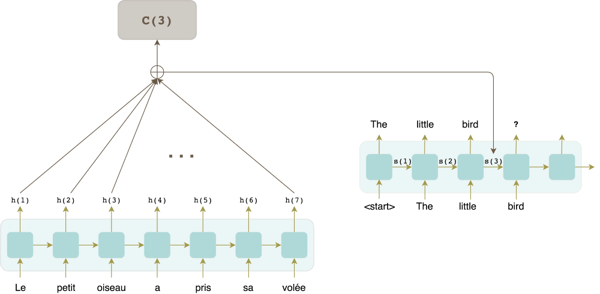
The model needs to weight all the words in the input sentence, giving more importance to words that relate the most to the word the model is about to predict and using the information it has on hand, which in this case is the last decoder hidden state s(3). This vector represents a summary of all the words decoded so far and can be seen as the closest thing to the word the model is about to predict. Following this intuition, the weight for input word j is computed as a “similarity” measure between its hidden state vector and the vector s(3):

Step 1: For each encoder hidden state h(j), compute a “similarity” measure between this vector and s(i-1), the last decoder hidden state.
Function a can be an arbitrary function in theory. In practice, Bahdanau et al. used a single layer feed forward neural network.
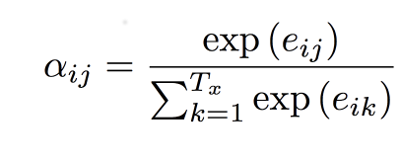
Step 2: These weights are then passed through a Softmax layer.
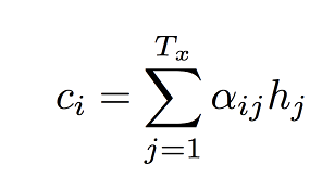
Step 3: And then used to weight the hidden state vectors.
The resulting context vector c(i)is then used in the decoder (along with the previous decoder hidden state and the last predicted word) in order to generate the next word.
 This is only one type of attention, which is called additive attention. Other forms of attention have been proposed since. The Luong multiplicative attention mechanism is one example worth noting.
The Blessing of Soft Alignment
Here is a cool property that you get when using attention: the model learns by itself the alignment of words between the input words and the output words. Which also makes for a great inspection tool:
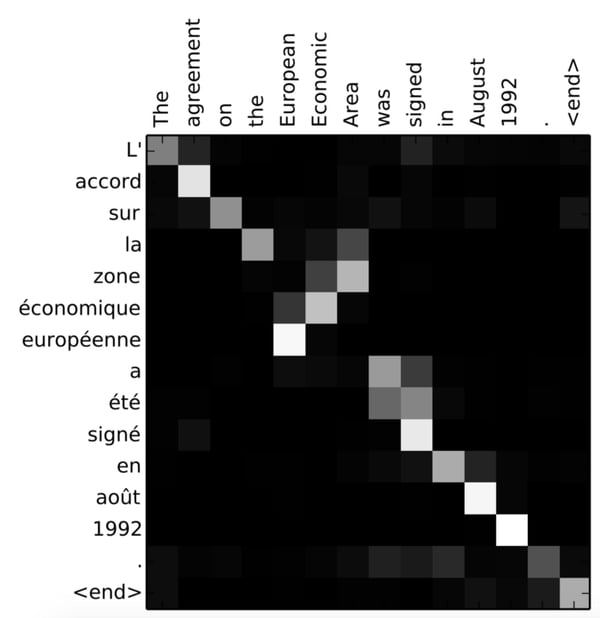 Heatmap showing the values of the attention wights for English to French translation. Source: https://arxiv.org/pdf/1409.0473.pdf
As you can see, the alignment is pretty much monotonic with the exception of certain cases, such as the expression: European Economic Area, where the order of the words in the French translation is reversed (zone économique européenne); the model is able to look back and forth to focus on the right word.
Conclusion
This was the very first time where an attention mechanism was successfully applied to machine translation, and it opened the door for different architectures that leverage this technique in some way or another. One of these architectures drastically changed the NLP game and set it on a path into a new area: the Transformer. Stay tuned, as the next post in this series will be about exactly that, the transformer architecture!
