


We saw how attention works and how it improved neural machine translation systems (see the previous blog post). We are now going to unveil the secrets behind the power of the most famous NLP models nowadays (a.k.a BERT and friends), the Transformer. In this second part, we are going to dive into the details of this architecture with the aim of getting a solid understanding of how its different components operate and interact.

Attention Everywhere!
As you now understand, attention was a revolutionary idea in sequence-to-sequence systems such as translation models. The folks of the Google Translate team understood this very well. Being full of ideas (and GPUs), these people had the amazing idea to push attention even further.
This boiled down to this rather simple observation: In addition of using attention to compute representations (i.e., context vectors) out of the encoder’s hidden state vectors, why not use Attention to compute the encoder’s hidden state vectors themselves? The immediate advantage of leveraging this idea was appealing: Get rid of the inherent sequential structure of RNNs, which hinders the parallelization of such models.
As professor Eugenio so eloquently put it:
Drop your RNN and LSTM, they are no good!… Forget RNN and variants. Use ATTENTION. ATTENTION really is all you need! ”
And so in 2017, in their now iconic paper Attention Is All You Need, the world was introduced to this new architecture:
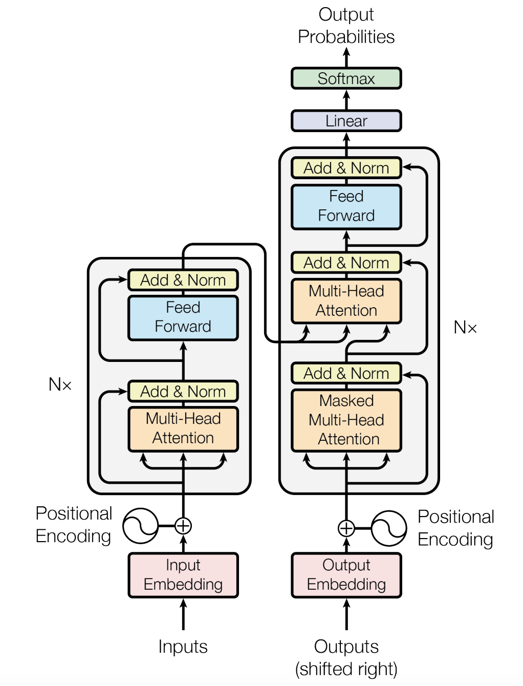
In this blog, we will shed some light into the main components of this model.
As the saying goes “You don’t change a winning team.” Consequently, the core concepts of the previously discussed model were kept: The transformer leverages an encoder-decoder architecture as well as an attention mechanism between these two components. But not only that: In the following, we are going to discuss the self-attention layer, the multi-head concept, and the magic of positional encodings.
Self-Attention
Let’s now get down to the central component, the self-attention layer (called multi-head attention in figure 1; we will get to the reason behind this name in a moment). Self-attention is first and foremost a sequence-to-sequence transformation, meaning it transforms a sequence of tokens into a new sequence of tokens.
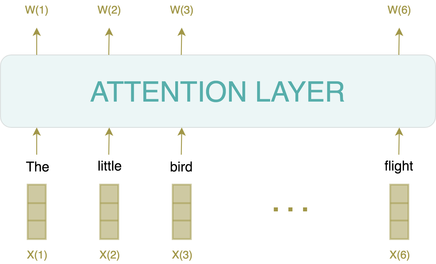
As we now understand, a good representation of a word needs to consider its context within a sentence (this is already one of the core ideas of ELMo, for instance). In other words, the representation vectorW(i) of word i needs to account for the wordsW(1),...,W(i-1)left of i and similarly, wordsW(i+1),...,W(n) right of i. This entails being somehow able to relate a word with its neighboring words. Which takes us to the second idea, which is commonly used in machine learning: how do you assess how related two items are? Two Amazon products, two Netflix viewers…or two words in a sentence? You usually take their dot product (in an appropriate space):
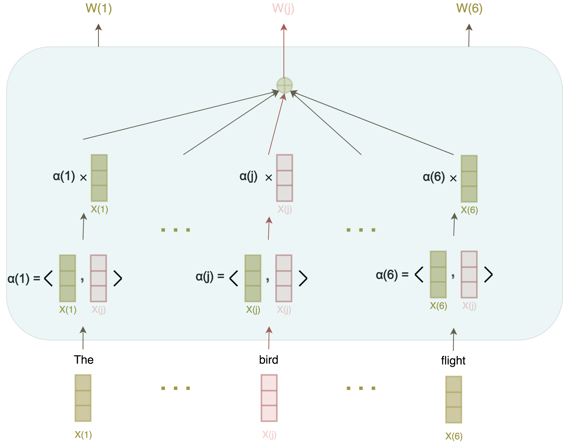
And voilà, self-attention in its bare-bones version. In order to get to a more complete version, we need to clear the air around two things:
- First, what do the
X(i)vectors look like? What do you feed the self-attention layer, i.e., what are the initial representations of each word in the sentence? Well, these can be computed in several ways. For instance, you can use the good old tf-idf, or you can keep up with NLP fashion and use word embeddings (GloVe, Fasttext, or Word2vec, for example). - Second, what does related words really mean? Lot of things! For example, two words in a sentence can be related with a subject-to-verb relation (the words “bird” and “has” share this relation). Ideally, we would like that the dot product between the embeddings of these two words — and all the words that share the same grammatical relation — to be high, and inversely, to be low for words that don’t share this grammatical relation. The bad news is that your out-of-the-box pre-computed word embeddings were not trained to answer this specific question. The good news is that we can still leverage these pre-computed embeddings and fine-tune them as part of the whole transformer training.
Three Embeddings for the Price of One
Now let’s take a step back and think of how the embedding W(i) of word ineeds to behave. Here, I want you to notice that this single vector is actually being used in three different tasks! (In the following, I am paraphrasing this blog post):
1- To compute the new representation of word i: The embedding W(i) will be used in the dot product with the other wordsW(j)of the sentence to compute the weights for each word.
2- To compute the new representations of the other words in the sentence j: The embedding W(i) will be used in the dot product with these words to compute the weights for each word.
3- To compute the new representation of word i: The embedding W(i) will be used as a summand of the final weighted sum.
Here we come to yet another genius idea of this paper. Instead of learning for each word one single embedding to perform these three tasks, why not learn a different word embedding for each task? Going from a general-purpose embedding to three specialized embeddings for each word. We will call the embedding for task 1 the query, for task 2 the key, and for task 3 the value.
Let us now revisit figure 3:
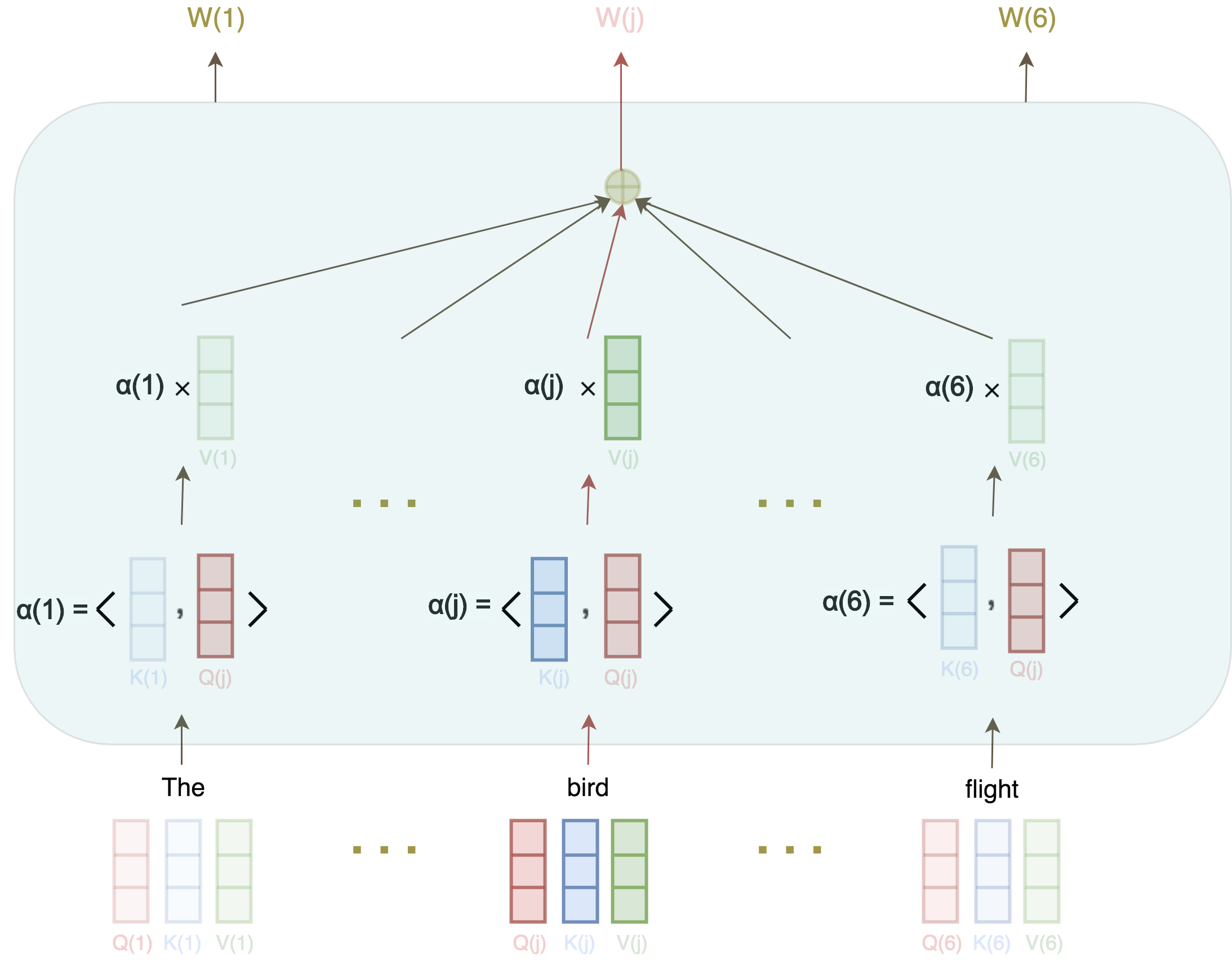
Say we want to compute the attention representation of the word “bird.” First, we measure how this word is related to all the other words in the same sentence: The little bird took its flight.
We do this by taking the dot product of its Query vector, Q(bird), with the Key of all the other words, K(the),...,K(flight), yielding a vector of weights for all the words in the sentence: α(the),…,α(flight). We then use these weights in the weighted sum of Value vectors of all the words in the sentence V(the),...,V(nest).

And since all of these operations are independent, they can be vectorized:
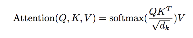
This really is the gist of it! I have deliberately omitted a few details of the true implementation (such as the normalizing constant, the feed-forward layer, the residual connections, etc.). I invite you to read the original paper to cover these. If you’d like more details around the Query, Key, and Value parameters, I encourage you to check out Jay Alammar’s great blogpost on transformers.
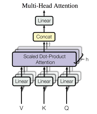
The Icing on the Cake: Multi-Head Attention
“Well hold on,” you might say. “I get that we need to train new embeddings to capture the subject-to-verb relation, but what about other relations that might exist?” Nice catch. After all, you might also want to infer that “bird” and “its” are related through the possessive-to-noun relation.
The solution to this problem is simple: For each word, create as many different embeddings as there are relations we may want to capture. This translates to having multiple parallel self-attention layers instead of only one. This is called multi-head attention.
A Final Call to Order: Positional Encodings
You might notice that we did not mention for one moment the order of the words in a sentence. This is expected; the self-attention operation is permutation invariant. That is, it will yield the same results not matter how you permute the words within a sentence. But this of course did not prevent the authors from establishing some order in the mess.
The authors propose to present this information to the model by adding an embedding vector of dimension d_model, a vector of the same size, to each word. This positional encoding vector would, in theory, tell the model about the position of this word within the sentence. Let us first state these vectors.

As an example, the positional encoding vector of the word bird in the sentence: The little bird took its flight (here we take d_model=300),is:

We can also have a look at a heatmap of positional encodings of a longer sentence (the sentence was generated using the infamous GPT-2 model). Each row corresponds to a word and displays the 40 first values of its positional encoding vector.
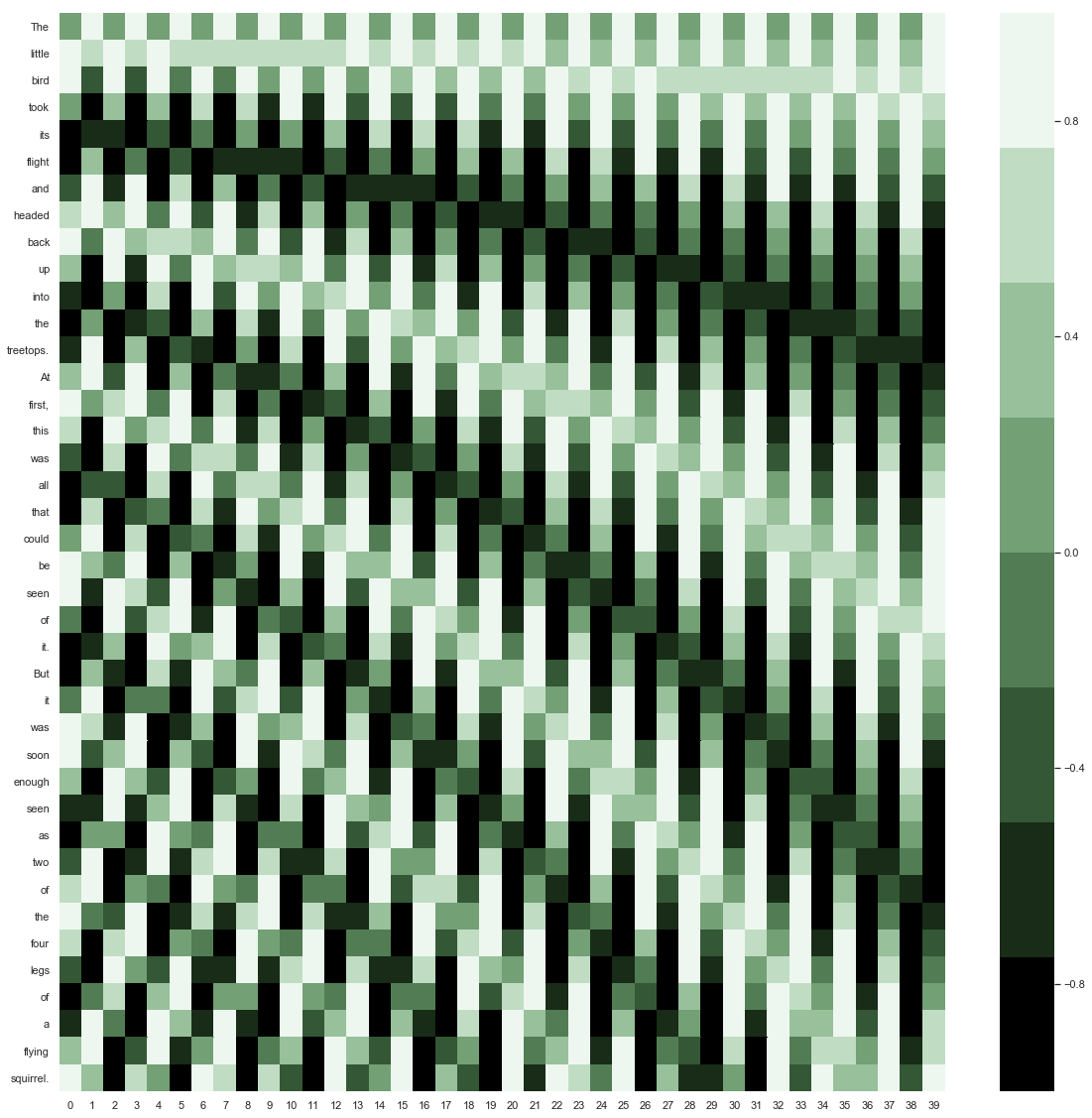
So how can we make sense of these vectors? In order to understand the logic behind them, let’s analyze two fundamental properties that these vectors need to follow:
…it may allow the model to extrapolate to sequence lengths longer than the ones encountered during training. [Attention is all you need]
This means that even if the model was trained on sentences no longer that N words, it should be able to correctly score longer sentences. This steered the choice of these encodings towards periodic functions and helped settle on these family of functions rather than training these positional encoding vectors from scratch.
We hypothesized it would allow the model to easily learn to attend by relative positions, since for any fixed offset k, PE(pos+k) can be represented as a linear function of PE(pos). [Attention is all you need]
One fundamental property that these vectors need to have is that they should not encode the intrinsic position of a word within a sentence (“The word took is at position 4”), but rather the position of a word relative to other words in the sentence (“The word took is at position 3, relative to the word the”).
In other words, if the distance between two words A and B in a sentence is the same as between words C and D, their positional encoding vectors should reflect that fact. It turns out that the aforementioned function family follows this property. If you are curious, check out the proof in this blog post.
Conclusion
We set the road through this blogpost and the previous one toward grasping the magic behind the most recent and most famous NLP models out there. In the next blogpost, we are going to shed the light to one of the first models that successfully leveraged the transformer architecture: BERT.