Recommendation Engines (In Plain English!)

In the previous posts in the In Plain English! series, we went through a high-level overview of machine learning and have explored two key categories of supervised learning algorithms — linear and tree-based models — and two key unsupervised learning techniques, clustering and dimensionality reduction. Today, we’ll dive into recommendation engines, which can use either supervised or unsupervised learning.

At a high level, recommendation engines leverage machine learning to recommend relevant products to users. You probably use recommendation engines every day for things like shopping suggestions, movie recommendations, dating app matches, and more (without even realizing it!). 

Brands gather lots of data on how users behave. Recommendation engines are very useful for suggesting products to users. These recommendations are crucial in driving user engagement and ensuring that users come back to your store or service. Companies commonly use recommendation engines for B2C purposes, but they can also utilize them for other purposes.

There are many ways to create recommendation engines, and the best method depends on your dataset and business objectives. Let’s dive into each of them.

Recommendation Engines in Action: Practical Examples

Imagine you own Willy Wonka's Candy Store. You could launch an email marketing campaign. This campaign would use AI to suggest personalized candy choices for each user.

Then, imagine all customers rate candies from 1-5. We want to recommend candies to George.

Most recommendation algorithms store the key data in a dataset called a utility matrix, as shown in Figure 1. The utility matrix contains past purchase behavior or ratings for each individual user and product combination. Typically, the goal of a recommendation engine is to predict the unknown values and recommend products with high predicted values for an individual user.

Figure 1

This is a simple example, but a utility matrix is typically very large and sparse as users will likely only have reviewed or interacted with a small subset of products. For example, most customers at the candy store will not have tried or rated every product, and most users on Netflix have not seen every movie. This sparsity will come into play when we evaluate different approaches.

Also note that we have explicit rating data here, or, this is an explicit recommendation engine. Many times we only have implicit data such as past purchases or likes, which we’ll use as a proxy for rating data, represented as zeros and ones.

There are two key methods of generating recommendations programmatically:

1. Content-Based Filtering
2. Collaborative Filtering

Let’s dive into specific applications of each method.

Content-Based Recommendation Engines

Content-based recommendation engines use product information in order to recommend items to a user that are similar to the items that the user liked in the past . If we were recommending songs, we might look at the genre, artist, length, or song lyrics, for example.

In order to do this for George, we must create an item vector for each item in our dataset and a user vector summarizing George’s preferences. Item vectors contain features describing each of our items. In this example, the item vectors might contain information like ingredients, calories, candy category, and so on, as represented for Twix in Figure 2.

Twix Item Vector

Figure 2

George User Vector

Figure 3

From the item vectors of the candies George liked, we can infer a user vector, or the features of candies that George likes. The simplest method generates a weighted average of the item vectors, where candies that George likes more are weighted more heavily. From George’s user vector, we can see that George tends to skew towards chocolate candies, and is less of a fan of gelatin-based candies, such as gummy bears.

Once we’ve generated a user vector, we can compute the similarity between the user vector and each of the item vectors. Several distance metrics can be used, but the most common is cosine similarity. Cosine similarity measures the size of the angle between two vectors, and values range from -1 to 1, where:

• -1 indicates an angle close to 180°, or opposite vectors
• 0 indicates an angle close to 90°, or unrelated, orthogonal vectors
• 1 indicates an angle close to 0°, or identical vectors

We can visualize this concept if we imagine each vector existing in a two-dimensional space, with only two features (see Figure 4). Because the angle (θ) between George’s user vector and the Milky Way item vector is small, we have a high cosine similarity and can predict that George will like Milky Ways.

There’s an orthogonal — or perpendicular — relationship between George’s user vector and the Tootsie Roll item vector, indicating that George would likely feel indifferent about Tootsie Rolls. Lastly, the very obtuse angle between George’s user vector and the Starburst item vector indicates that George would probably dislike Starbursts.

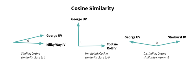Figure 4

After computing similarities between George’s user vector and item vectors for all candies that he has not yet purchased, we’ll then sort these candies in order of similarity and recommend the top N candies, or the “nearest neighbors.” In Figure 5 below, we can see that George likes the green candies which have similar features to the blue candies, which he has not yet purchased, so the blue candies might be a good product to recommend.

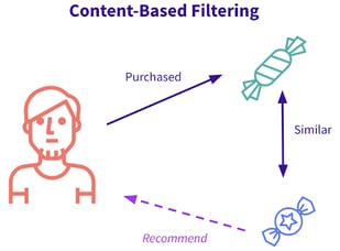Figure 5

This is a quite simple example; we’ll often work with more complex data types such as text or image data for a content-based recommendation problem. To convert text or image data into something a machine can understand, we must vectorize it, or convert it into a numerical format, once it has been cleaned and pre-processed. There are many forms of vectorization, but that is beyond the scope of this post. See here for a bit of detail on Natural Language Processing (NLP) and vectorization.

Note that there are also other methods of generating content-based recommendations, such as building a traditional classification (to predict likes) or regression model (to predict rating value), clustering to find similar items, or deep learning for even more sparse datasets like image data, but the nearest-neighbors based approach is one of the most classic and commonly used methods.

There are several advantages to content-based filtering. This approach:

• Doesn’t require data on other users
• Can generate recommendations for new & unpopular items as well as users with unique tastes
• Has a relatively straightforward interpretation

Disadvantages of this approach include:

• Difficulty extracting all relevant information, as user tastes are complex and users are not often loyal to a specific candy category or movie genre, etc.
• Limitations, as it can only recommend products similar to past purchases
• The cold start problem for new users (no prior rating information)

Collaborative Filtering

Collaborative filtering deals with the first two disadvantages nicely, as we’ll look at past rating patterns rather than product information. This is based on the assumption that users have specific tastes, and past rating patterns are all we need in order to predict future ratings.

There are two key methods of collaborative filtering:

1. Memory-Based Filtering
2. Model-Based Filtering

Memory-Based Methods (User-Based & Item-Based)

Memory-based methods use data directly from the utility matrix to find "near neighbors," which can represent either similar users or similar items, depending on the axis considered. If recommendations are made along the user axis, recommendations are user-based and if they’re made along the item axis, they’re item-based. Let’s explore each method.

User-Based

The user-based method rests on the assumption that people who’ve liked many of the same products in the past have similar taste, and that this can be used to infer preferences. For example, if Jen likes strawberry lollipops, sour apple hard candies, and blueberry hard candies, and George likes sour apple hard candies and pink lollipops, we may want to recommend blueberry hard candies to George.

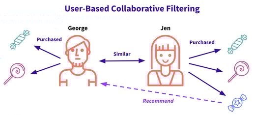
Figure 6

Here’s how it works:

1. Compute similarities between George and all other customers in the dataset. This similarity metric (cosine similarity, Pearson’s correlation, etc.) measures the similarity between rows in our utility matrix, or, how frequently the two customers rate candies similarly.
2. Predict ratings for all candies that George has not yet tried. Predicted ratings are a weighted sum of past user ratings for each candy. Ratings by users very similar to George will be weighted more heavily, and vice versa.
3. Recommend top candies by sorting all candies by highest predicted rating to lowest and recommend the top N.

This approach is relatively simple, but is fairly time consuming and computationally expensive, as we need to compute similarities between each combination of users in our dataset. If our dataset has many more users than items, computing similarities between items can be more efficient. This leads us to item-item collaborative filtering.

Item-Based

Rather than finding similarities between users, with item-based collaborative filtering, we’ll find similarities between items. For example, let’s imagine we know the below:

• Jerry likes sour apple hard candies, strawberry lollipops, and orange candy canes.
• Jen likes sour apple hard candies, strawberry lollipops, and blueberry hard candies.
• George likes apple hard candies.

We can infer that sour apple hard candies are likely similar to strawberry lollipops, as we saw that both Jerry and Jen liked both of them, and since we only now know that George likes sour apple hard candies, this might be a good product to recommend.

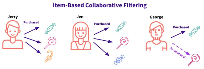Figure 7

Here’s how we generate these recommendations:

1. Compute similarities between all items in the dataset. This captures similarity in past user ratings among candies, or, similarity among columns in our dataset.
2. Predict ratings for all candies that George has not yet tried. To predict what George will rate grape lollipops, we’d get a weighted sum of George’s past ratings, where candies more similar to grape lollipops are weighted more heavily.
3. Recommend top candies by sorting all candies by highest predicted rating to lowest and recommend the top N.

Overall, memory-based methods tend to be fairly straightforward, but require a lot of time and computational resources. Item-based tends to be a bit more effective than user-based as items are simpler than users and often belong to specific categories, whereas users often have very complex and unique tastes. Item-based is also typically more efficient as a dataset typically has fewer items than users, but to scale out for a very large dataset, a model-based method is typically a better approach.

Model-Based

The most common model-based methods leverage matrix factorization, a family of dimensionality reduction algorithms aimed at decomposing a matrix into two or more smaller matrices. This rests on the assumption that sparse datasets tend to consist of a handful of latent, or hidden, features, and rather than looking at every item in our dataset, we can project these items into several latent categories, and the same goes for users.

For example, candies in a certain category, such as chocolate candies or gelatin-based candies, may tend to have similar rating patterns. Each of these categories would be considered latent features, and rather than looking at each individual candy, we can group all candies within a category into one column. The categories are often not as clearly defined as this, so a model-based dimensionality reduction approach is typically the best way to discern the latent categories that exist within a dataset.

We can decompose our utility matrix into two smaller matrices, one which captures all customers and latent candy features and another which captures all candies and latent customer features. In Figure 8 below, customers and candies each have two latent features.

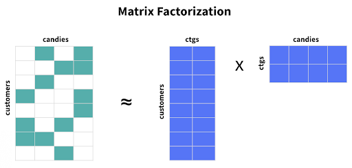Figure 8

There are a handful of methods of generating these matrices. Singular Value Decomposition (SVD) and Non-Negative Matrix Factorization (NMF) are two of the most common decomposition algorithms for recommender systems. There are two key methods of optimizing values in the user and item matrices: Alternating Least Squares (ALS) and Stochastic Gradient Descent (SGD). The math behind these algorithms is beyond the scope of this introductory post, but the principal idea is that we’ll decompose one matrix into two smaller ones which capture key latent features.

Once we have converted our utility (customer*candy) matrix into user (customer) and item (candy) matrices, we can multiply these two smaller matrices together to approximate the missing values in the utility matrix. Again, we’ll sort predicted ratings for candies that George has not yet tried, and recommend the top N.

While dimensionality reduction obscures interpretability, matrix factorization tends to generate the strongest predictions of all methods listed, as reducing the dimensionality reduces overfitting, and we are no longer beholden to the restraints of content-based methods. Additionally, memory consumption is greatly reduced by shrinking the size of the matrices we’re working with, and focusing on the key latent factors.

This said, all collaborative filtering algorithms share some key problems:

• Cold start problem - We don’t have past rating information for new users or new products. There are several ways of remedying this problem. For new products, we can use a content-based system or draw attention to them with a “new releases section,” and for new users we may start with something as simple as most popular items until we collect more information. Nonetheless, it’s a clear drawback.
• Sparsity & computational complexity - Even with matrix factorization, we may still run into memory consumption issues if we’re working with very large datasets. In this situation, we’ll typically turn to distributed computing via Spark or Hadoop.
• Popularity bias - Items that are often rated highly will likely have high predicted ratings for users, and niche items will not be frequently recommended.

Recap

Recommendation engines are an excellent way for brands to keep customers engaged by recommending relevant content. There are many methods of generating recommendation engines, each with its own set of pros and cons.

Content-based recommender systems use user rating history along with product information to identify products similar to those a particular user liked in the past. This is fairly straightforward and works well in recommending new and unpopular products. However, this approach is often a bit too simplistic.

Collaborative filtering does not consider product information at all, and relies strictly on the utility matrix, containing past rating information for all users and products, to find similar users and recommend products that they liked. Memory-based collaborative filtering methods are fairly simple, but often don’t scale well for large datasets. Model-based methods build upon this by leveraging dimensionality reduction to improve memory consumption. Even so, memory consumption is still a common drawback, as is the cold start problem and popularity bias.

Note that these two approaches are not mutually exclusive, and hybrid approaches are common. One example of a hybrid approach is using a content-based system for new products, and a collaborative filtering model for products that we have more rating history on.

Recommendation engines are an extensive topic, and there’s much more to it than what is mentioned here, but we hope you found this introduction to the topic insightful.